Hierarchical ordinal regression for analysis of single subject data OR Bayesian estimation of overlap and other effect sizes

Background

I’ve been interested in analysis of single case designs (SCD) using hierarchical models: each case is unique but we can improve estimation for each case by sharing data across cases. Given that data from SCD are often atypical, I’ve thought such data are a good candidate for ordinal regression.¹

Broadly, we can model unidimensional² continuous, count, ordinal data as ordinal, since these data are also ordinal. If we knew the exact distribution for the data, we could perform more efficient analyses, but we often don’t. Frank Harrell often recommends this kind of ordinal approach and provides several resources here. There are also useful papers: here³, here⁴, and here⁵, and I’ve applied to same idea to analysis of sum scores of Likert-response scales.⁶

Given this interest, I did some work on ordinal hierarchical models for analysis of SCD some time back – time stamp on my laptop says January 2022!! This work never left my laptop, and I mentioned it in passing to maybe two people. I thought of reaching out to James Pustejovsky to get his thoughts, but for some reason, I didn’t follow through.

Enter AERA 2024, I somehow found myself at a structured poster session for analysis of SCD. Very interesting work all around; count mixed models, model-based effect size estimation and benchmarks, single case mediation, … Made me want to share this again, and James P. encouraged me to send it his way. So here goes.

Description of hierarchical ordinal model

I focus on simple designs: AB, ABAB, …

I originally did this work with splines for approximating ordinal thresholds e.g.⁵, and splines for modeling case-specific trajectories. But I settled for something more conventional in the SCD literature.

The model assumes case-specific intercepts and treatment effects, and I use hierarchical modeling to estimate both. Additionally, the data within each case are autocorrelated.

First step is to transform the data to (dense) ranks.

Multivariate normal model for unobserved continuous data given observed ordinal data

If we assume ordinal data were originally normal data that have been discretized and we attempt to build a regression for the original normal data, we arrive at probit regression. Following Albert & Chib (1993)⁷, we can use this relation to model multivariate ordinal data with multivariate probit regression. This allows us set a correlation structure on the ordinal data at the latent level.

Model

Assume the latent data for case $c\in \{1,\dots ,C\}$ is a $T$-dimensional vector, $z_c$. $z_c$ are sampled as truncated variables given the constraints imposed by the ordered threshold-vector, $\kappa$. I represent the treatment indicator variable for case $c$ as $x_c$, then the hierarchical ordinal model is:

$$\begin{array}{cc}& z_c\sim N_T({\gamma }_c+{\beta }_c\times x_c,\Sigma ),\\ & {\gamma }_c\sim N(0,{\tau }_0),{\beta }_c\sim N(b_0,{\tau }_1),\\ & b_0\sim N(0,{\tau }_b),[{\tau }_0,{\tau }_1,{\tau }_b]\sim t^{+}\left(3\right),\kappa \sim t\left(3\right)\end{array}$$

where ${\gamma }_c$ is intercept for case $c$ shrunken towards 0. Since we will estimate all ordinal thresholds, the grand-mean is 0. The case-specific treatment effect, ${\beta }_c$, is shrunken towards $b_0$, and $b_0$ is itself shrunken towards 0 (akin to a ridge regression penalty).

I set up the elements of the covariance matrix, ${\sigma }_{i,j}$, as:

$${\sigma }_{i,j}={\varphi }^{|i-j|},\frac{\varphi +1}{2}\sim \text{beta}(5,5)$$

such that $\varphi$ is the autocorrelation coefficient. The prior on $\varphi$ assumes a 95% chance $\varphi$ falls in the $(-.6,.6)$ interval – this sounds like a good choice.⁸ The diagonal elements of the matrix are fixed to 1 for the purpose of identifying the probit model.

Effect sizes

The ordinal probit model above is one for the cumulative distribution function (CDF) of the ranks. From there, we compute the probability mass function (PMF). Given the PMF, one can then apply several of the equations listed in the documentation of the SingleCaseES package to obtain effect sizes. I focus on the NAP, PEM and TAU (since it’s just $2\times$ NAP - 1). For effects defined on the original data scale like differences in means or medians, we can simply replace ranks with the original data to obtain results on the original data scale. We can obtain uncertainty intervals for all effects since we compute each effect size within each posterior iteration.

R code

I implemented the model above with Stan. The code is available as a gist file and contains two demonstrations. I review the demonstrations below.

Demonstrations

Tasky (2008)⁹

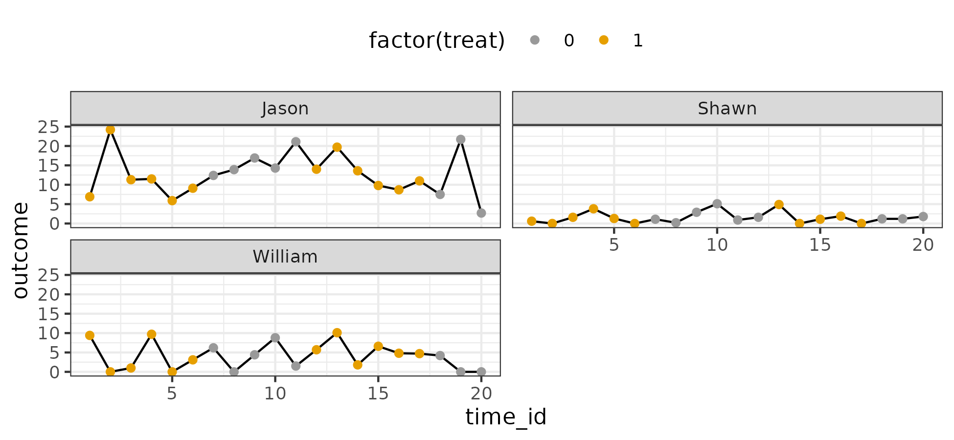
I visualize the data below:

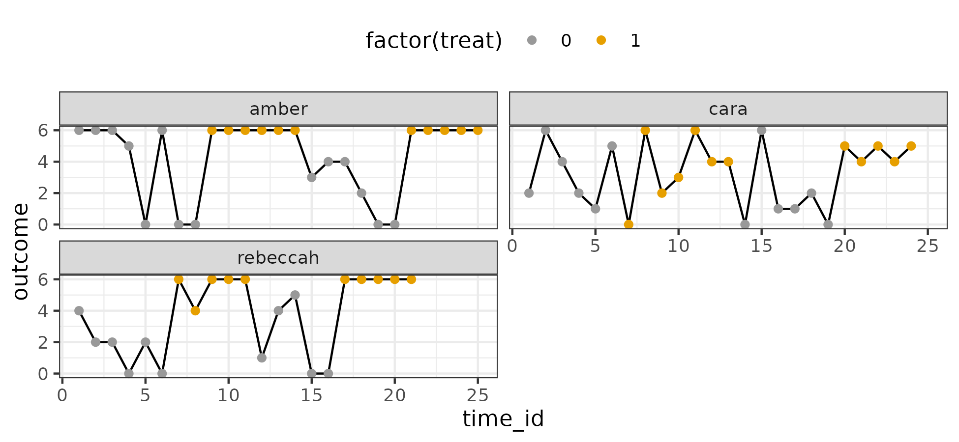
There are three cases. The outcome is a count variable with 7 unique values – easy to assume an ordinal model. Higher values are desirable.

I fit the model, parameters appeared to converge without significant problems. For posterior predictive checking, I assessed the proportion for each count (95% intervals):

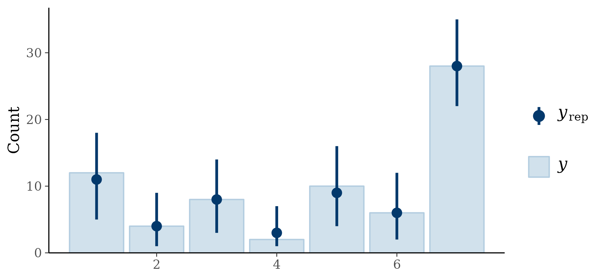
Results look acceptable. I also plotted the posterior predictive distribution against the individual trajectories on the ordinal scale (90% intervals):

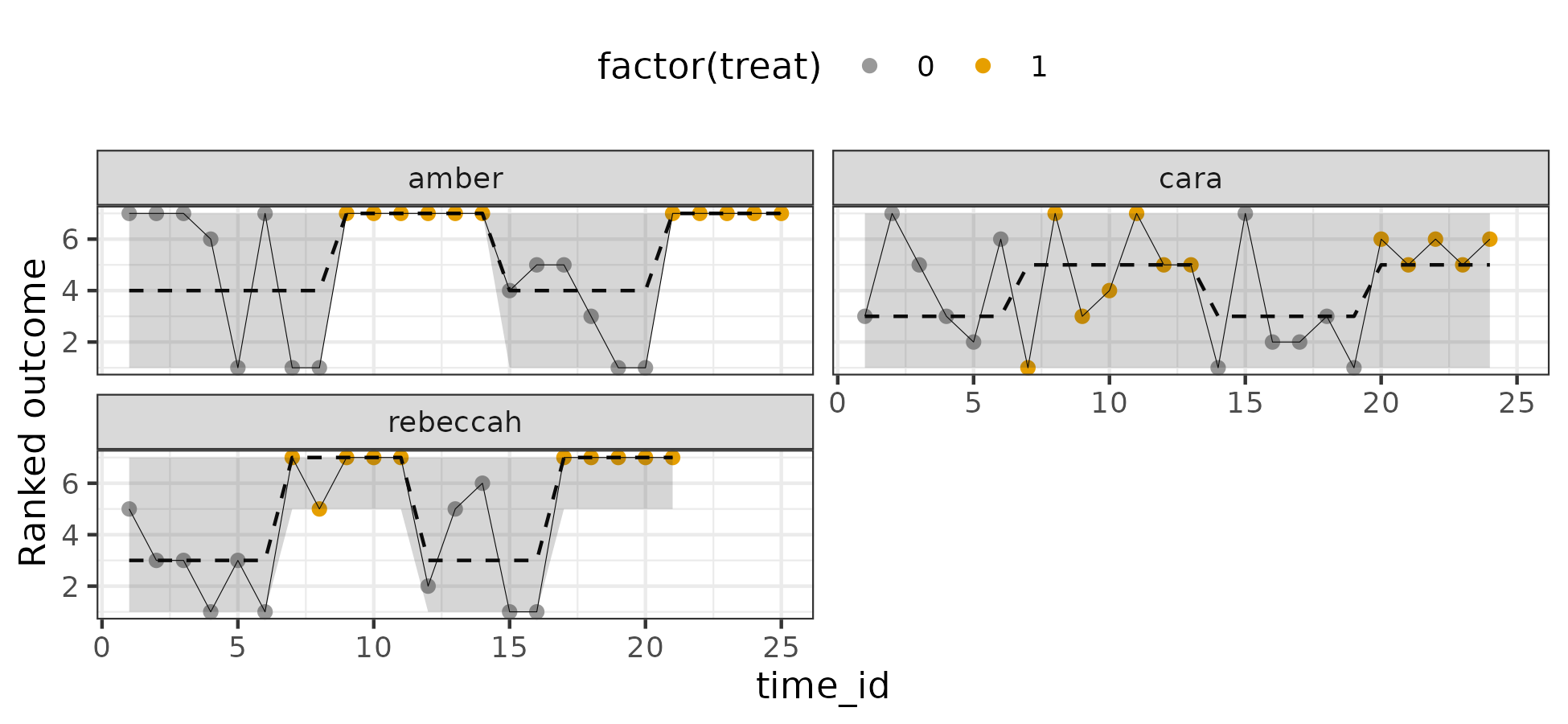
Also looks reasonable. Now for effects (intervals are 80% and 95%):

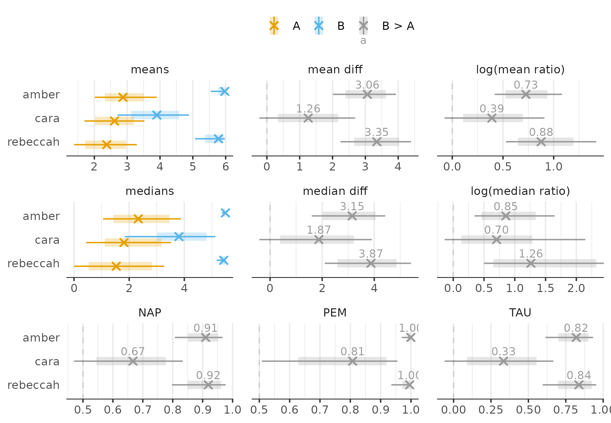
Regardless of the effect size, there is improvement for Amber and Rebeccah but the evidence is not as conclusive for Cara. Only the PEM provides clear evidence of improvement for Cara, but the uncertainty about the 81% estimate is still large.

Then I compare the ordinal model effects to simple case-wise computations obtained from the SingleCaseES package (95% intervals):

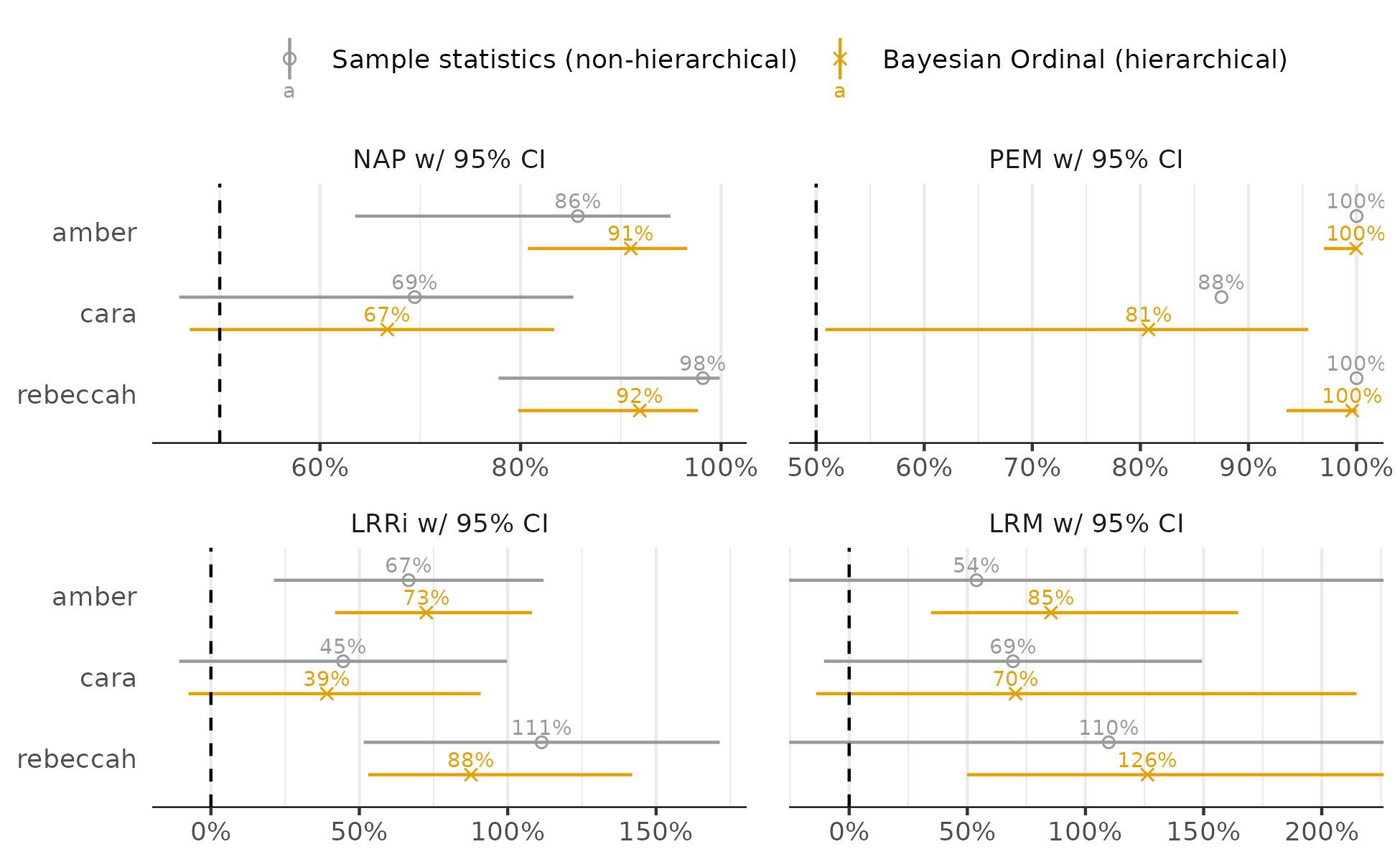
The ordinal model-based effects often have less uncertainty and are often shrunken – effects of pooling and regularization. This makes the most difference for the log-ratio of medians estimates (LRM) where the improved conclusions for Amber and Rebeccah are more certain in the ordinal analysis. Note that LRRi is the log-ratio of means. Also, the sampling distribution of the PEM is not yet known, the ordinal model helps with that.

Schmidt (2012) from SingleCaseES package

I visualize the data below:

There are three cases. The outcome is seemingly continuous and has 48 unique values. Again, higher values are desirable.

I fit the model, parameters appeared to converge without significant problems. For posterior predictive checking, I compared the density of the observed data to the density of draws from the posterior predictive distribution:

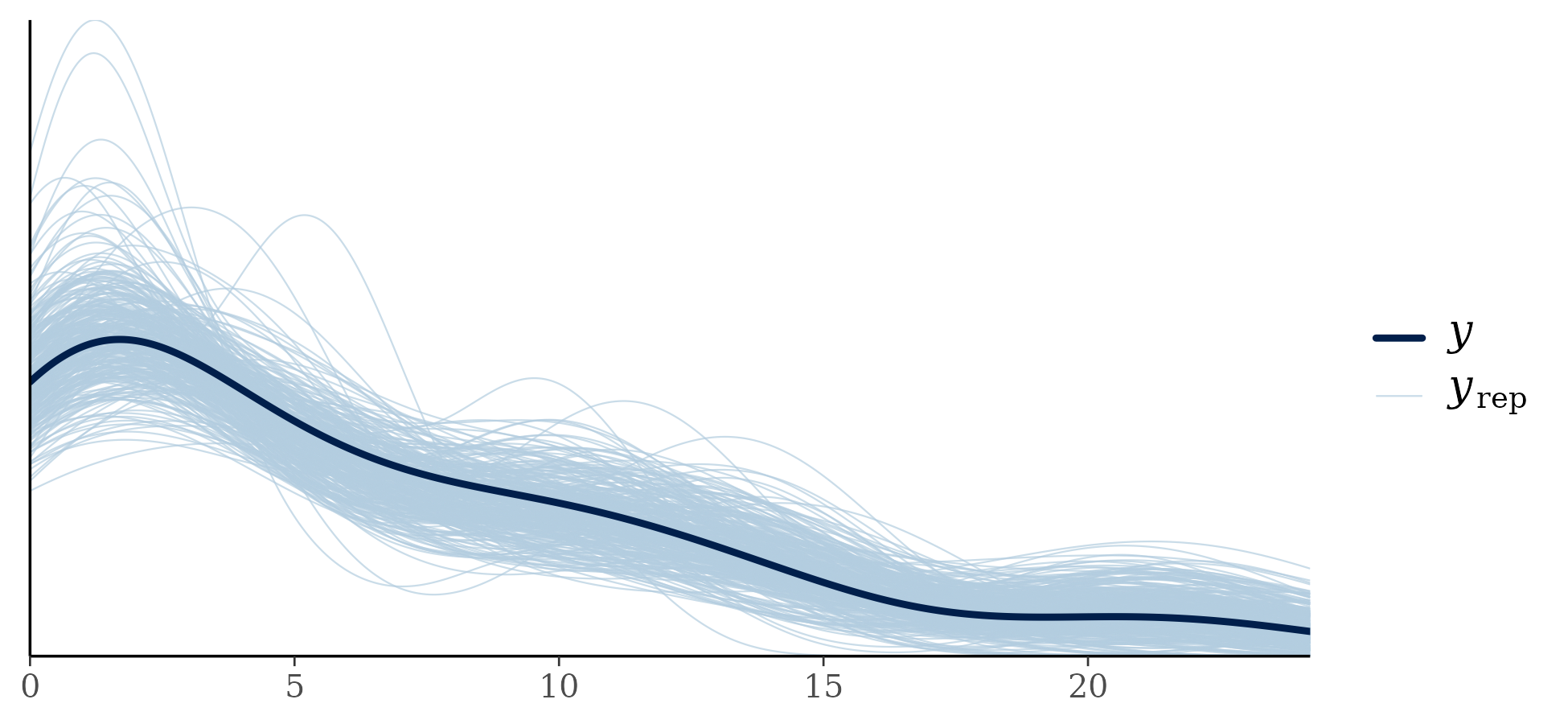
These results are on the original data scale, though they could be examined on the ordinal scale. For the original data scale, I replace the ranks in the posterior predictive distribution with the original values that were rank transformed. Results look acceptable – an advantage of the ordinal approach is that pretty much any distributional shape is realizable.

I also plotted the posterior predictive distribution against the individual trajectories on the ordinal scale (90% intervals):

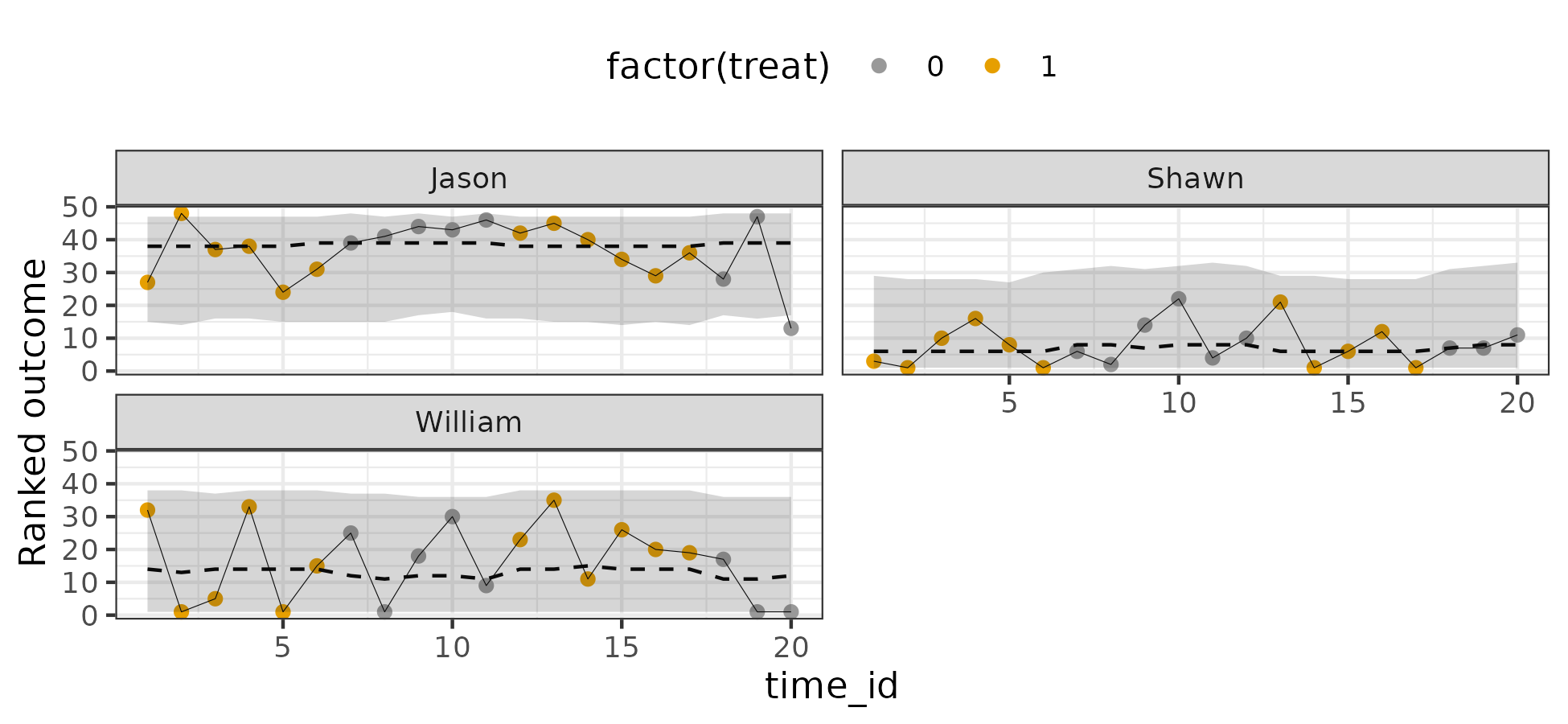
We see a fairly flat pattern. This suggests the treatment hardly made a difference.

Now for effects (intervals are 80% and 95%). I exclude mean and median ratios – I think these are usually count related metrics:

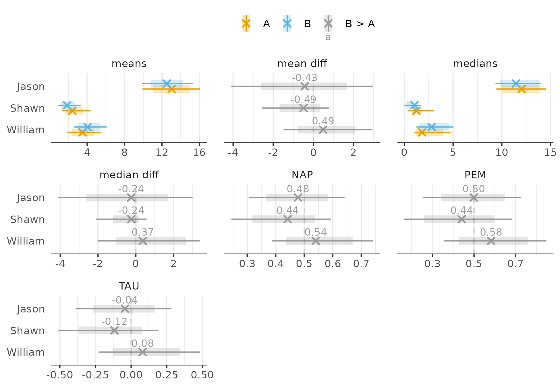
None of the effects provide strong evidence for improvement.

Then I compare the ordinal model effects to the standard approach (95% intervals):

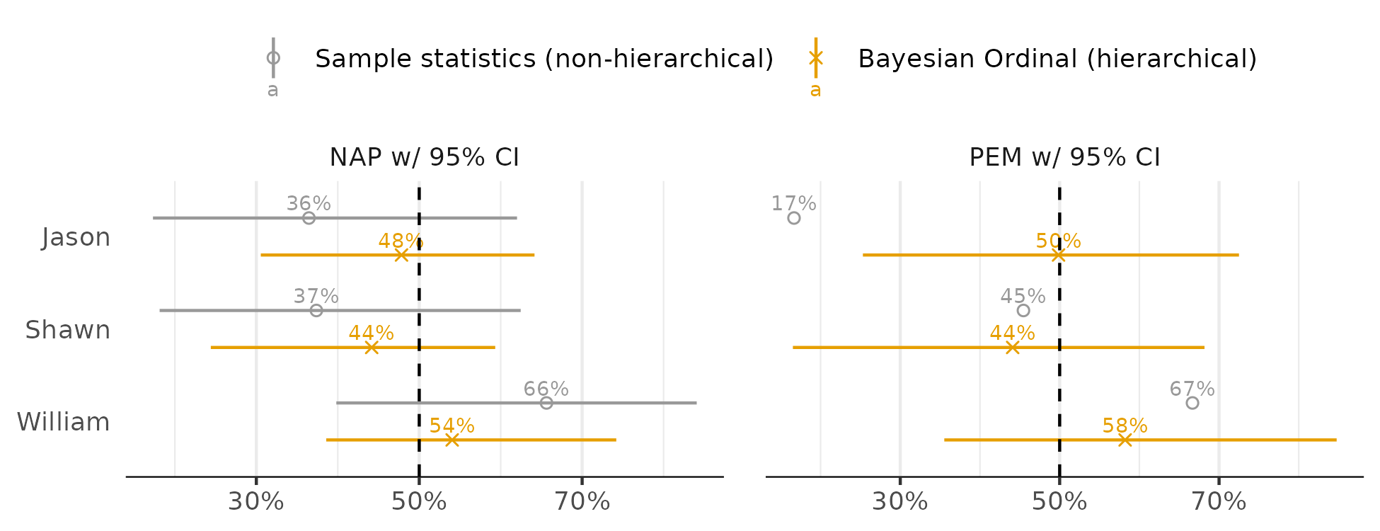
We again see more stable coefficients for the ordinal approach. The most notable difference between approaches is Jason’s PEM. The standard approach returns 17% while the ordinal approach returns 50%. If you check the raw data, we can see that most of Jason’s intervention points are lower than the median of the control values. However, we would also be unlikely to conclude the intervention made things worse for Jason – the pattern looks like much fluctuation, no meaningful change. And the 17% PEM seems misleading about the overall patterns in the data.

In closing

I think ordinal regression can be pretty useful for analyzing SCD data. It’s no coincidence that several of the effect sizes used to support visual analysis of trajectories are ordinal effect sizes. The gist above contains the code to create all these plots and other plots I did not mention here. I tried to comment the scripts well enough, so I hope the gist is helpful.

Some notes about the model

• I assumed no correlation between the random intercept and random treatment effect – no strong thoughts about this but I noticed with some examples that the posterior for this parameter often just matched the prior and I didn’t want to think about it much.
• The priors are stand-in defaults, they require more thought than I’ve put into them at this stage.
• In limited trials, model runtime depends on the number of thresholds (in addition to the amount of data which is not usually much for SCD). But when using a spline to approximate the thresholds, the number of parameters can be held constant. See this gist for some examples of using splines to approximate the thresholds, though I do not account for autocorrelation in these models. Instead, I have case-specific trajectories.
• Trying to capture autocorrelation on the latent scale is the reason for the multivariate normal approach. One could instead predict the current ordinal level using the previous ordinal level, see here for examples by Frank Harrell.