Should you perform logistic regression on a dichotomized continuous variable when you have access to the continuous variable? I’m not sure.

See here for an update, I recommend not dichotomizing, but it pays to read this first.

A standard situation in education or medicine is we have a continuous measure, but then we have cut-points on those continuous measures that are clinically/practically significant. An example is BMI where I hear 30 matters. You may have an achievement test with 70 as the pass score. When this happens, researchers may sometimes be interested in modeling BMI over 30 or pass/fail as the outcome of interest. The substantive question often falls under the lines of modeling the probability of someone exceeding/falling short of this clinically significant threshold. So we dichotomize the continuous measure and analyze the new binary response using something like logistic regression.

Going back to intro stats, you hear things like: “don’t dichotomize your predictors, you’ll throw away information/variance/power …”. Of course the same applies to outcomes, and most people would rather a regular linear regression than logistic regression. However, in the scenario above, we often justify dichotomizing the outcome for substantive reasons.

I came across a 2004 Stats in Medicine paper by Moser and Coombs¹ with the title, “Odds ratios for a continuous outcome variable without dichotomizing” almost a year ago now. I only read it closely more recently. The authors reiterate the point that you throw away information when you dichotomize the outcome. And they show that you don’t really need to dichotomize the outcome to obtain the odds ratios. The nice thing about the paper is that until they get into the equations that span several lines, the paper is easy to follow. Here’s the summary:

1. You believe that \(\alpha + X\beta + \epsilon = y_c\), where \(y_c\) is a continuous outcome i.e. some variables, \(X\), multiplied by their coefficients, \(\beta\), plus the intercept, \(\alpha\), and some error, \(\epsilon\), result in your continuous outcome, \(y_c\).
2. You believe that some threshold \((t)\) is clinically significant, so you cut \(y_c\) at \(t\) such that all values of \(y_c\) exceeding \(t\)are now 1 and all others are 0; we’ll call this new variable \(y_b\).
3. You then perform logistic regression on \(y_b\), which really is just an attempt to retrieve the original model, \(\alpha + X\beta + \epsilon = y_c\). Why not directly model \(y_c\)?

A few points are worth making about this:

1. We can summarize the above as: $$y_b = 1 \quad \mathrm{if}\quad \alpha + X\beta + \epsilon > t \quad \mathrm{otherwise}\quad y_b = 0$$.
2. If we adjust the threshold, say drop it by 1 point, it does not change \(X\beta\), it only affects the intercept: $$y_b = 1\quad \mathrm{if}\quad \alpha - 1 + X\beta + \epsilon > t - 1$$
3. The point here it that the only coefficient affected by changing the threshold is the intercept, \(\alpha\); the \(\beta\)are not affected by adjusting the threshold. So the relationships we do care about are not affected by the threshold – more on this later.
4. Finally, in logistic regression, we do not estimate \(\epsilon\), we assume it is standard logistic. That affects things such that if we want to use the linear regression on \(y_c\)to obtain the results from logistic regression, we need to make some adjustments.²

So here’s what they recommend:

• Estimate the linear model on the continuous outcome, \(y_c\)
• Your coefficients are \(\beta\), then transform them: $$\frac{\pi}{\sigma\times\sqrt{3}}\beta\quad\text{where }\sigma = \text{ residual standard deviation of regression}$$
• These are your log odds, you can exponentiate them to obtain odds ratios.
• We do not care for the intercept from this linear regression because it will be affected by the threshold, and we are using an approach that is blind to the threshold.

So how does this approach work in practice? Anyone who has tried dichotomizing a continuous variable at different thresholds prior to analysis using logistic regression will know that the estimated coefficients do change and they can change a lot! Is this consistent with the claim that the result should not be dependent on the thresholds? We can check using simulation. First, I walk through the data generation process:

set.seed(12345) # Set seed for reproducible results

# Our single x variable is binary with 50% 0s and 50% 1s
# so like random assignment to treatment and control
# Our sample size is 300
dat <- data.frame(x = rbinom(300, 1, .5))
# Outcome ys = intercept of -0.5, the coefficient of x is 1 and there is logistic error
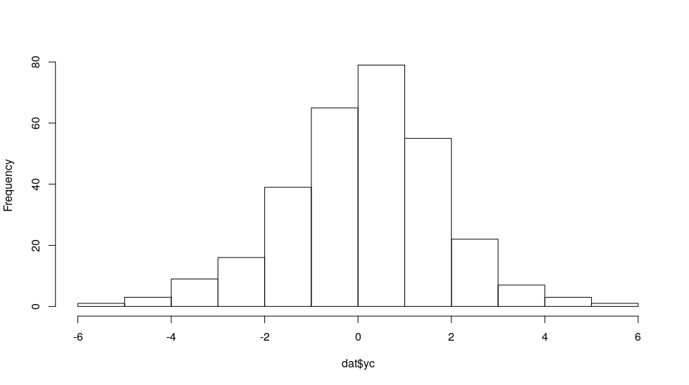
dat$yc <- -.5 + dat$x + rlogis(nrow(dat))

yc looks something like:

hist(dat$yc, main = "")

We can then dichotomize the yc outcome at various points to see whether that affects the estimated coefficient of x when we use logistic regression:

coef(glm((yc > -2) ~ x, binomial, dat))["x"] # Cut it at extreme -2
        x
0.9619012

coef(glm((yc > 0) ~ x, binomial, dat))["x"] # Cut it at midpoint 0
       x
1.002632

coef(glm((yc > 2) ~ x, binomial, dat))["x"] # Cut it at extreme 2
        x
0.8382662

So the numbers are a little different. What if we applied the linear regression to yc directly?

# First, we create an equation to extract the coefficients and
# transform them using the transform to logit formula above.
trans <- function (fit, scale = pi / sqrt(3)) {
  scale * coef(fit) / sigma(fit)
}
trans(lm(yc ~ x, dat))["x"]
       x
1.157362

All these numbers are not too different from each other. If we exponentiate them to obtain odds ratio, they’d be more different. Now we can repeat this process several times to compare the patterns in the results. I’ll repeat it 2500 times:

colMeans(res <- t(replicate(2500, {
  dat <- data.frame(x = rbinom(300, 1, .5))
  dat$yc <- -.5 + dat$x + rlogis(nrow(dat))

  # v for very; l/m/h for low/middle/high; and t for threshold; ols for regular regression
  c(vlt = coef(glm((yc > -2) ~ x, binomial, dat))["x"],
    lt = coef(glm((yc > -1) ~ x, binomial, dat))["x"],
    mt = coef(glm((yc > 0) ~ x, binomial, dat))["x"],
    ht = coef(glm((yc > 1) ~ x, binomial, dat))["x"],
    vht = coef(glm((yc > 2) ~ x, binomial, dat))["x"],
    ols = trans(lm(yc ~ x, dat))["x"])
})))
    vlt.x      lt.x      mt.x      ht.x     vht.x     ols.x
1.0252116 1.0020822 1.0049156 1.0101613 1.0267511 0.9983772

These numbers are the average regression coefficients for the different methods.

v stands for very, l/m/h stand for low/middle/high and t stands for threshold, ols is the regression result. So for example, vlt.x is the average x coefficient from the very low threshold model.

These estimated coefficients average to about 1 for all methods, which is what we programmed, good! How variable is each method?

boxplot(res)

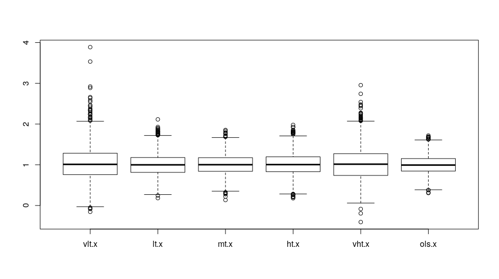
We see that although the averages are about the same, when the threshold is extreme, the estimated coefficients are more variable. The least variable coefficients are the transformed linear regression coefficients, so when we use the linear regression approach, the result is somewhat stable. The more extreme the thresholds are, the more variable coefficients we’ll get. This is interesting because we often dichotomize data for logistic regression at the extremes.

How about the pattern of estimated coefficients between the different methods?

GGally::ggpairs(as.data.frame(res))

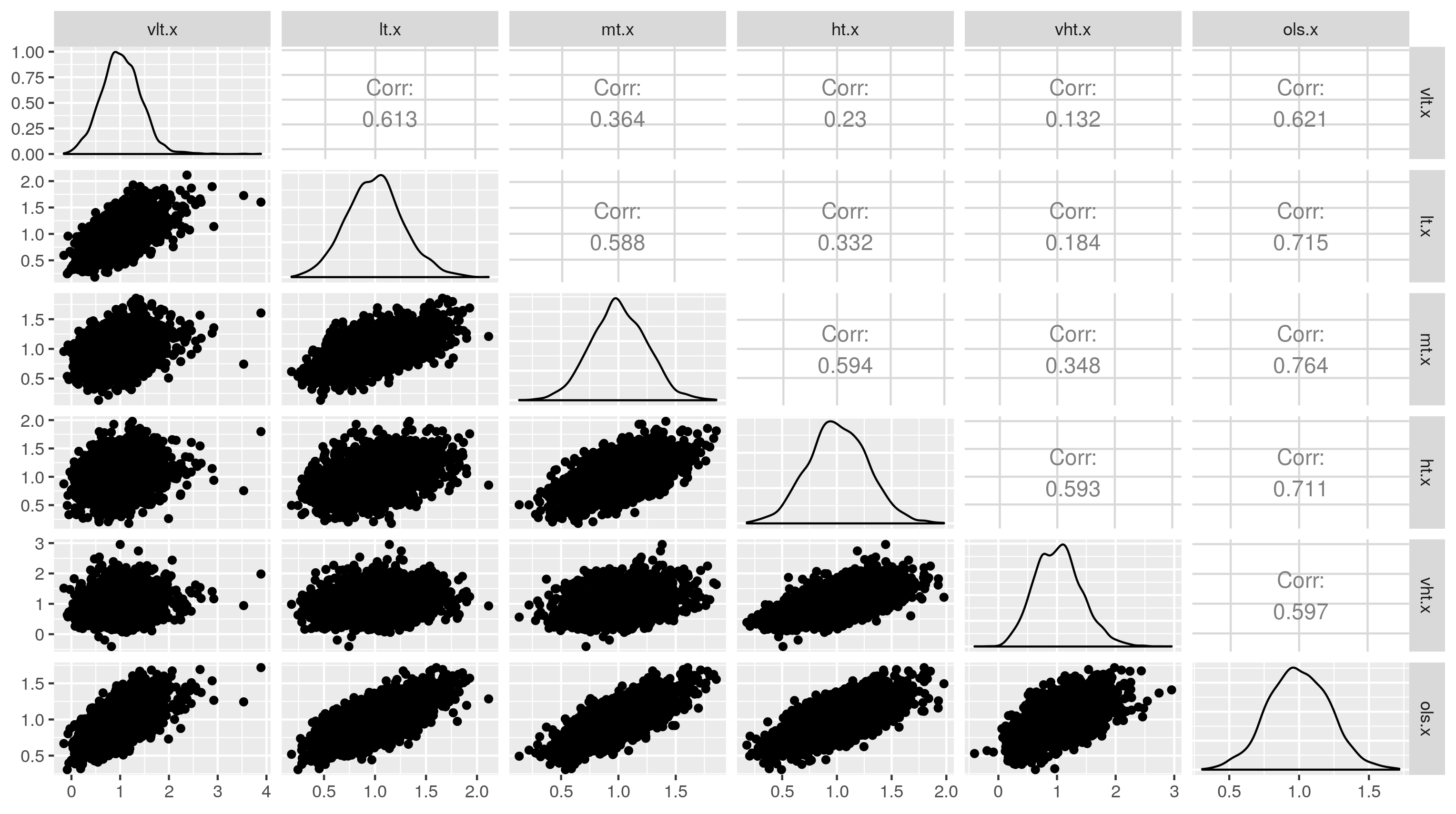
We see that although all the methods claim x has a coefficient of 1 with y on average, the estimated coefficient when the threshold is very low is very weakly correlated with the estimated coefficient when the threshold is very high (.13). These are differences simply reflect the threshold and can be misleading in actual data analysis. One may believe widely different estimates at different thresholds represent different population parameters (true coefficients) when they do not. The method with which each method is most highly correlated is the linear regression method. The linear regression method is most strongly correlated with the middle threshold results. It is also the most stable and does not appear to be biased.

Based on these results, one may believe that we should always model the continuous variable then transform our coefficients using Moser and Coombs' formula if we want the log odds and/or odds ratio. Moser and Coombs reached that conclusion.

Substantively, should we trust the findings when the data are dichotomized at extreme thresholds? Or should we just go with the transformed linear regression coefficient?

It is also possible that the relationship between the predictors and the outcome is different at different quantiles of the outcome – a situation quantile regression explores. One can use a quantile regression approach to see if this exists in the original continuous outcome.³