Simulating data from regression models

My preferred approach to validating regression models is to simulate data from them, and see if the simulated data capture relevant features of the original data. A basic feature of interest would be the mean. I like this approach because it is extendable to the family of generalized linear models (logistic, Poisson, gamma, …) and other regression models, say t-regression. It’s something Gelman and Hill cover in their regression text.¹ Sadly, the default method of simulating data from regression models in R misses what one might consider an important source of model uncertainty - variance in estimated regression coefficients.

Your standard regression model assumes there are true/fixed parameters relating the predictors to the outcome. However, when we perform regression, we only estimate these parameters. Hence, regression software returns standard errors which represent coefficient uncertainty. All other things being equal, smaller sample sizes lead us to greater coefficient uncertainty meaning larger standard errors. The default method for simulating data from a model ignores this uncertainty. Is this a big problem? Maybe not so much. But it would be nice if this source of model uncertainty was not ignored.

I’ll demonstrate what I mean using an example.

Demonstration

I’ll use Poisson regression to demonstrate this. I simulate two predictors, one continuous, xc, and one binary, xb. And use a small sample size of 50.

library(MASS) # For multivariate normal distribution, handy later on
n <- 50
set.seed(18050518)
dat <- data.frame(xc = rnorm(n), xb = rbinom(n, 1, .5))

Coefficient will be .5 for xc and 1 for xb. I exponentiate the prediction and use the rpois() function to generate a Poisson distributed outcome.

# Exponentiate prediction and pass to rpois()
dat <- within(dat, y <- rpois(n, exp(.5 * xc + xb)))
summary(dat)

       xc                  xb             y       
 Min.   :-2.903259   Min.   :0.00   Min.   :0.00  
 1st Qu.:-0.648742   1st Qu.:0.00   1st Qu.:1.00  
 Median :-0.011887   Median :0.00   Median :2.00  
 Mean   : 0.006109   Mean   :0.38   Mean   :2.02  
 3rd Qu.: 0.808587   3rd Qu.:1.00   3rd Qu.:3.00  
 Max.   : 2.513353   Max.   :1.00   Max.   :7.00  

Next is to run the model.

summary(fit.p <- glm(y ~ xc + xb, poisson, dat))

Call:
glm(formula = y ~ xc + xb, family = poisson, data = dat)

Deviance Residuals:
    Min       1Q   Median       3Q      Max  
-1.9065  -0.9850  -0.1355   0.5616   2.4264  

Coefficients:
            Estimate Std. Error z value Pr(>|z|)    
(Intercept)  0.20839    0.15826   1.317    0.188    
xc           0.46166    0.09284   4.973 6.61e-07 ***
xb           0.80954    0.20045   4.039 5.38e-05 ***
---
Signif. codes:  0 ‘***’ 0.001 ‘**’ 0.01 ‘*’ 0.05 ‘.’ 0.1 ‘ ’ 1

(Dispersion parameter for poisson family taken to be 1)

    Null deviance: 91.087  on 49  degrees of freedom
Residual deviance: 52.552  on 47  degrees of freedom
AIC: 161.84

Number of Fisher Scoring iterations: 5

The estimated coefficients were not too distant from the population model, .21 for the intercept instead of 0, .46 instead of .5, and 0.81 instead of 1.

Next to simulate data from the model, I’d like 10,000 simulated datasets because why not? To capture the uncertainty in the regression coefficients, I assume the coefficients arise from a multivariate normal distribution with the estimated coefficients acting as means and the variance-covariance matrix of the regression coefficients as the variance-covariance matrix for the multivariate normal distribution.²

coefs <- mvrnorm(n = 10000, mu = coefficients(fit.p), Sigma = vcov(fit.p))

Out of curiosity, I check how well the simulated coefficients match the original coefficients. First the means:

coefficients(fit.p)

(Intercept)          xc          xb
  0.2083933   0.4616605   0.8095403

colMeans(coefs) # means of simulated coefficients

(Intercept)          xc          xb
  0.2088947   0.4624729   0.8094507

Pretty good, and next the standard errors:

sqrt(diag(vcov(fit.p)))

(Intercept)          xc          xb
 0.15825667  0.09284108  0.20044809

apply(coefs, 2, sd) # standard deviation of simulated coefficients

(Intercept)          xc          xb
 0.16002806  0.09219235  0.20034148

Also pretty good.

Next step is to simulate data from the model. We do this by multiplying each row of the simulated coefficients by the original predictors. Then we pass the predictions to rpois() so it generates a Poisson distributed response:

# One row per case, one column per simulated set of coefficients
sim.dat <- matrix(nrow = n, ncol = nrow(coefs))
fit.p.mat <- model.matrix(fit.p) # Obtain model matrix
# Cross product of model matrix by coefficients, exponentiate result,
# then use to simulate Poisson-distributed outcome
for (i in 1:nrow(coefs)) {
  sim.dat[, i] <- rpois(n, exp(fit.p.mat %*% coefs[i, ]))
}
rm(i, fit.p.mat) # Clean house

Now one is done with simulation, compare the simulated datasets to the original dataset on at least the mean and variance of the outcome:

c(mean(dat$y), var(dat$y)) # Mean and variance of original outcome

[1] 2.020000 3.366939

c(mean(colMeans(sim.dat)), mean(apply(sim.dat, 2, var))) # average of mean and var of 10,000 simulated outcomes

[1] 2.050724 4.167751

The average mean of the simulated outcomes was a little higher than that of the original data, the average variance was much higher. On average, one can expect the variance to be more off target than the mean. The variance will also be positively skewed with some extremely high values, at the same time, it is bounded at zero, so the median might be a better reflection of the center of the data:

median(apply(sim.dat, 2, var))

[1] 3.907143

The median variance is much closer to the variance of the original outcome.

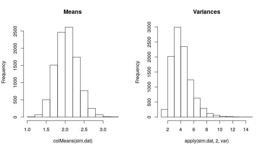
Here’s the distribution of the simulated means and variances:

par(mfrow = c(1, 2))
hist(colMeans(sim.dat), main = "Means")
hist(apply(sim.dat, 2, var), main = "Variances")
par(mfrow = c(1, 1))

The above is how I would simulate data from a model and conduct basic checks. It could also be useful to plot histograms of a few of the 10,000 simulated datasets and compare those to a histogram of the original outcome. One could also test the mean difference on the outcome between xb = 1 and xb = 0 in the original data and in the simulated datasets. If the data were over-dispersed, variance comparisons as done above or looking at a few histograms would reveal the inadequacy of a Poisson model if capturing the variance was important. Whatever features the investigator considers important can be examined and compared in this manner.

Back to base R, it has a simulate() function for doing the same thing:

sim.default <- simulate(fit.p, 10000)

This code is equivalent to:

sim.default <- replicate(10000, rpois(n, fitted(fit.p)))

fitted(fit.p) is the prediction on the response scale, or the exponentiated linear predictor since this is Poisson regression. Hence, we’d be using the single set of predicted values from the model to repeatedly create the simulated outcomes.

What does it suggest about recovery of data features:

c(mean(colMeans(sim.default)), mean(apply(sim.default, 2, var)),
  median(apply(sim.default, 2, var)))

[1] 2.020036 3.931580 3.810612

The mean and variance are closer to the mean and variance of the original outcome than when one ignores coefficient uncertainty. This approach will always result in a lower variance than when one considers the uncertainty in regression coefficients. It is much faster and requires zero programming to implement, but I am not comfortable ignoring uncertainty in regression coefficients, making the model seem more adequate than it is.

Another problem is most packages that utilize lm() and glm() and simulate data from the model would probably not implement their own simulate() function. For example, DHARMa, a great package for simulation-based residual diagnostics, also relies on the simulate() function when evaluating GLMs.