Modeling the error variance to account for heteroskedasticity

One of the assumptions that comes with applying OLS estimation for regression models in the social sciences is homoskedasticity, I prefer constant error variance (it also goes by spherical disturbances). It implies that there is no systematic pattern to the error variance, meaning the model is equally poor at all levels of prediction.

This assumption is important for OLS to be the best linear unbiased predictor (BLUE). Heteroskedasticity, the complement of homoskedasticity, does not bias OLS, however, it causes it to be inefficient, losing the “best” property in the BLUE. If you do not care for p-values unlike most in the social sciences, then heteroskedasticity may not be an issue.

Econometricians have developed a whole variety of heteroskedasticity-consistent standard errors, so they can continue to apply OLS (which continues to be unbiased), while adjusting for non-constant error variance. The Wikipedia page on these corrections lists the many names these alternative standard errors go by.

Some time last semester, I was playing around with the mle() function in the stats4 package and also found the more versatile but slower mle2() in the bbmle package. We provide the likelihood function, and both functions will find the parameter estimates that maximize the likelihood. See footnote for additional details.¹

Let’s work through a quick example:

library(bbmle) # For the mle2 function
set.seed(180511)

First, I draw 500 observations from a normal distribution with mean 3 and standard deviation 1.5, and save it into a dataset:

dat <- data.frame(y = rnorm(n = 500, mean = 3, sd = 1.5))

The mean and standard deviation of the sample are:

mean(dat$y)
[1] 2.999048

sd(dat$y)
[1] 1.462059

I can also ask the question this way, what parameters of the normal distribution, mean and standard deviation, maximize the likelihood of this observed variable? The quick way to answer the question would be:

m.sd <- mle2(y ~ dnorm(mean = a, sd = exp(b)), data = dat,
             start = list(a = rnorm(1), b = rnorm(1)))

In the syntax above, I inform R that the mean of the variable y is a constant, a, and y’s standard deviation is a constant, b. The standard deviation is exponentiated ensuring it is never a negative number. We provide starting values, these are suggestions to the program so it can begin estimation prior to converging to a value that maximizes the likelihood. A random number would suffice for starting values.

m.sd

Call:
mle2(minuslogl = y ~ dnorm(mean = a, sd = exp(b)), start = list(a = rnorm(1),
    b = rnorm(1)), data = dat)

Coefficients:
        a         b
2.9990478 0.3788449

Log-likelihood: -898.89

The coefficient, a, looks very much like the mean of the data. You would have to exponentiate coefficient b, to obtain the standard deviation:

exp(coef(m.sd)[2])
       b
1.460596

This is similar to the standard deviation we got above. Another interesting fact demonstrated with the syntax above is lm() functions like coef() and summary() are available for use on mle2() objects.

The maximum-likelihood estimation we have performed above is similar to an intercept-only regression model estimated with OLS:

coef(lm(y ~ 1, dat))
(Intercept)
   2.999048

sigma(lm(y ~ 1, dat))
[1] 1.462059

The intercept is the mean of the data, and the residual standard deviation is the standard deviation.

Heteroskedastic regression models

Consider the following study. We have assignment two groups, a treatment group of 30 and a control group of 100 individuals matched to the treatment group on covariates that are determinants of the outcome. So we are interested in the treatment effect and let us assume a simple mean difference would suffice. It happens that the treatment in addition to being effective has a homogenizing effect, say the subjects were essentially brainwashed into doing better on the outcome. The following dataset should match the scenario above:

dat <- data.frame(
  treat = c(rep(0, 100), rep(1, 30)),
  y = c(rnorm(100), rnorm(30, 0.3, .25)))

There are 100 participants with 0 for treatment status (control group), they have a mean of 0 and a standard deviation of 1. There are 30 participants with 1 for treatment status (treatment group), they have a mean of 0.3 and a standard deviation of 0.25.

This scenario clearly violates the homoskedasticity assumption, nonetheless, we proceed with OLS estimation of the treatment effect:

summary(m.ols <- lm(y ~ treat, dat))

Call:
lm(formula = y ~ treat, data = dat)

Residuals:
    Min      1Q  Median      3Q     Max
-2.8734 -0.5055 -0.0287  0.4231  3.4097

Coefficients:
            Estimate Std. Error t value Pr(>|t|)
(Intercept)  0.03386    0.09298   0.364    0.716
treat        0.21733    0.19355   1.123    0.264

Residual standard error: 0.9298 on 128 degrees of freedom
Multiple R-squared:  0.009754,	Adjusted R-squared:  0.002018
F-statistic: 1.261 on 1 and 128 DF,  p-value: 0.2636

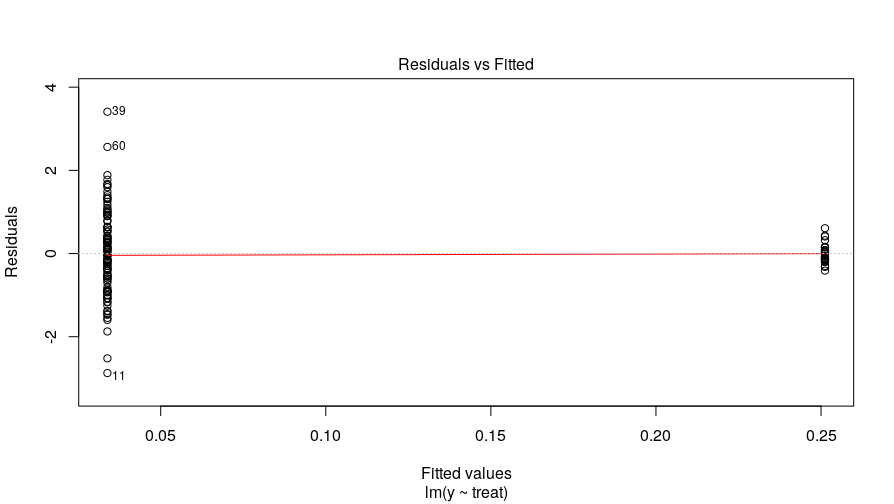
The treatment effect was .22 and not statistically significant, \(p = .26\) at an \(\alpha\)-level of .05. But we know the variances are not homoskedastic because we created the data and this simple diagnostic plot of residuals against fitted values confirms this:

plot(m.ols, 1)

We can address this using the mle2() function. First, I document the syntax to recreate the OLS model:

m.mle <- mle2(
  y ~ dnorm(mean = b_int + b_treat * treat, sd = exp(s1)), data = dat,
  start = list(b_int = rnorm(1), b_treat = rnorm(1), s1 = rnorm(1)))

In this function, I create a model for the mean of the outcome that is a function of an intercept, b_int, and a coefficient for the treat predictor, b_treat. The standard deviation is again an exponentiated constant. This model would be equivalent to the linear model.

However, we know the variances are not constant, but different for the two groups. We can instead specify the standard deviation as a function of the groups:

mle2(y ~ dnorm(mean = b_int + b_treat * treat,
               sd = exp(s_int + s_treat * treat)), data = dat,
     start = list(b_int = rnorm(1), b_treat = rnorm(1),
                  s_int = rnorm(1), s_treat = rnorm(1)))

Here, we have specified a model for the standard deviation as a function of an intercept, s_int, representing the control group, and a deviation from this intercept, s_treat.

We can do one better. We can use the coefficients from the OLS model as the starting values for b_int and b_treat. So I finally run the model:

summary(m.het <- mle2(
  y ~ dnorm(mean = b_int + b_treat * treat,
            sd = exp(s_int + s_treat * treat)), data = dat,
  start = list(b_int = coef(m.ols)[1], b_treat = coef(m.ols)[2],
               s_int = rnorm(1), s_treat = rnorm(1))))

Maximum likelihood estimation

Call:
mle2(minuslogl = y ~ dnorm(mean = b_int + b_treat * treat, sd = exp(s_int +
    s_treat * treat)), start = list(b_int = coef(m.ols)[1], b_treat = coef(m.ols)[2],
    s_int = rnorm(1), s_treat = rnorm(1)), data = dat)

Coefficients:
         Estimate Std. Error  z value   Pr(z)    
b_int    0.033862   0.104470   0.3241 0.74584    
b_treat  0.217334   0.112249   1.9362 0.05285 .  
s_int    0.043731   0.070711   0.6184 0.53628    
s_treat -1.535894   0.147196 -10.4344 < 2e-16 ***
---
Signif. codes:  0 ‘***’ 0.001 ‘**’ 0.01 ‘*’ 0.05 ‘.’ 0.1 ‘ ’ 1

-2 log L: 288.1408

The treatment effect is about the same, but the p-value is now .053. Much smaller than the .26 from the analysis assuming homoskedastic errors. The precision of the b_treat variable is much greater as the standard error here, .11, is smaller than .19.

The model for the standard deviation suggests a standard deviation of:

exp(coef(m.het)[3])

   s_int
1.044701

1.045 for the control group and:

exp(coef(m.het)[3] + coef(m.het)[4])

    s_int
0.2248858

.22 for the treatment group. These values are close to what we know we simulated. We can confirm the sample statistics as:

aggregate(y ~ treat, dat, sd)

  treat         y
1     0 1.0499657
2     1 0.2287307

It is also easy to conduct a model comparison of the model without heteroskedasticity and permitting heteroskedasticity:

anova(m.mle, m.het)

Likelihood Ratio Tests
Model 1: m.mle, y~dnorm(mean=b_int+b_treat*treat,sd=exp(s1))
Model 2: m.het, y~dnorm(mean=b_int+b_treat*treat,sd=exp(s_int+s_treat*treat))
  Tot Df Deviance  Chisq Df Pr(>Chisq)    
1      3   347.98                         
2      4   288.14 59.841  1  1.028e-14 ***
---
Signif. codes:  0 ‘***’ 0.001 ‘**’ 0.01 ‘*’ 0.05 ‘.’ 0.1 ‘ ’ 1

The likelihood ratio test suggests we have improved our model, \(\chi^2(1)=59.81,p<.001\).

So we can confirm that modeling the variance improves precision in this single example. It is easy to code a simulation comparing heteroskedastic MLE to OLS estimation when there is a null effect of zero and we have heteroskedasticity.

I make one change to the code from above by giving the treatment group a mean of zero, such that there is no mean difference between both groups. The treatment did not improve the outcome, but it homogenized people. I replicate the process 500 times saving the treatment effect from OLS and its p-value, and the treatment effect from heteroskedastic MLE, and its p-value.

res <- replicate(500, {
  dat <- data.frame(
    y = c(rnorm(100), rnorm(30, 0, .25)), treat = c(rep(0, 100), rep(1, 30)))
  m.ols <- lm(y ~ treat, dat)
  m.het <- mle2(
    y ~ dnorm(mean = b_int + b_treat * treat,
              sd = exp(s_int + s_treat * treat)), data = dat,
    start = list(b_int = coef(m.ols)[1], b_treat = coef(m.ols)[2],
                 s_int = rnorm(1), s_treat = rnorm(1)))
  list(b.ols = unname(coef(m.ols))[2],
       b.het = unname(coef(m.het))[2],
       p.ols = coef(summary(m.ols))[2, 4],
       p.het = coef(summary(m.het))[2, 4])
})
res <- apply(t(res), 2, unlist)

Then I plot the results:

par(mfrow = rep(2, 2))
for (i in 1:ncol(res)) {
  hist(res[, i], main = colnames(res)[i])
}
par(mfrow = c(1, 1))

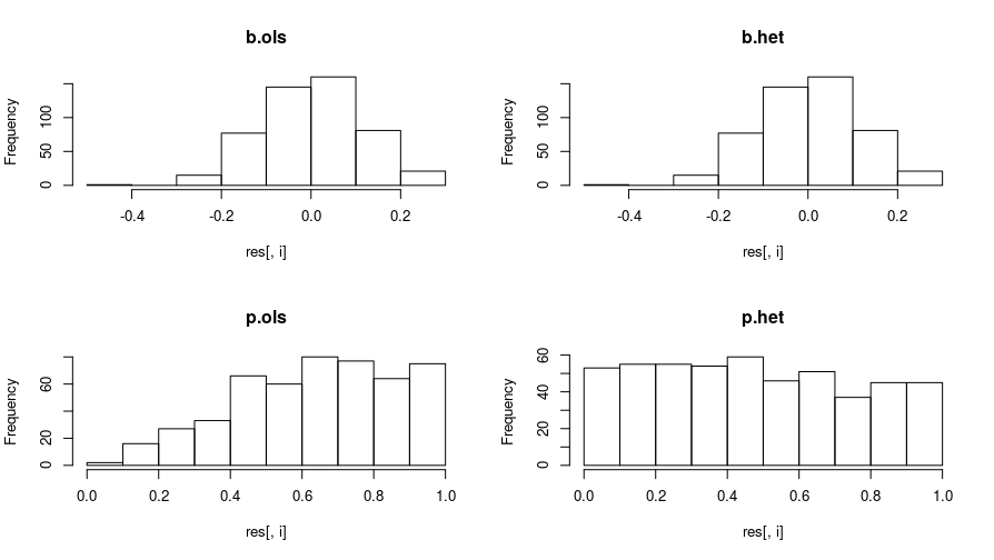
The treatment effects in the OLS and heteroskedastic MLE are similar. However, the p-values of the heteroskedastic MLE model are more well-behaved when the null is true. When the null is true, one would expect the p-values to be uniformly distributed. The p-values from the OLS iterations are stacked on the high end.

I repeat the process, this time, giving the treatment group a mean of .15, so the null of zero effect is false. And I get these plots:

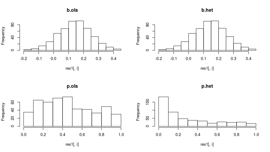
The treatment effects again have the same distribution. However, the p-values for the heteroskedastic MLE are much smaller, the heteroskedastic MLE has more statistical power to detect the treatment effect, compared to OLS.

The final syntax below breaks the process above down one level. It is the same syntax for the faster mle() function in the stats4 package. First, you specify a function for the negative log-likelihood (see ¹ below), then pass this function to MLE. Doing things this way allows for more transparency.

ll <- function(b_int, b_treat, s_int, s_treat) {
  with(dat, -sum(dnorm(
    y, mean = b_int + b_treat * treat,
    sd = exp(s_int + s_treat * treat), log = TRUE)))
}
summary(mle2(ll, start = list(
  b_int = rnorm(1), b_treat = rnorm(1),
  s_int = rnorm(1), s_treat = rnorm(1))))

Maximum likelihood estimation

Call:
mle2(minuslogl = ll, start = list(b_int = rnorm(1), b_treat = rnorm(1),
    s_int = rnorm(1), s_treat = rnorm(1)))

Coefficients:
         Estimate Std. Error  z value   Pr(z)    
b_int    0.033862   0.104470   0.3241 0.74584    
b_treat  0.217334   0.112249   1.9362 0.05285 .  
s_int    0.043733   0.070711   0.6185 0.53626    
s_treat -1.535893   0.147196 -10.4343 < 2e-16 ***
---
Signif. codes:  0 ‘***’ 0.001 ‘**’ 0.01 ‘*’ 0.05 ‘.’ 0.1 ‘ ’ 1

-2 log L: 288.1408

Alternatively, if one is interested in a solution that offers a bit more encapsulation, then one can use the glmmTMB package, and include a formula for the dispersion.

library(glmmTMB)
summary(glmmTMB(y ~ treat, dat, dispformula = ~ treat))

Family: gaussian  ( identity )
Formula:          y ~ treat
Dispersion:         ~treat
Data: dat

    AIC      BIC   logLik deviance df.resid
  296.1    307.6   -144.1    288.1      126


Conditional model:
           Estimate Std. Error z value Pr(>|z|)  
(Intercept)  0.03386    0.10447   0.324   0.7458  
treat        0.21733    0.11225   1.936   0.0528 .
---
Signif. codes:  0 ‘***’ 0.001 ‘**’ 0.01 ‘*’ 0.05 ‘.’ 0.1 ‘ ’ 1

Dispersion model:
           Estimate Std. Error z value Pr(>|z|)    
(Intercept)  0.08746    0.14142   0.618    0.536    
treat       -3.07179    0.29439 -10.434   <2e-16 ***
---
Signif. codes:  0 ‘***’ 0.001 ‘**’ 0.01 ‘*’ 0.05 ‘.’ 0.1 ‘ ’ 1

In this situation, the dispersion is on the scale of the log variance, so one would have to square root the exponentiated group log variances to retrieve the group standard deviations above.