I’ve been interested in the relationship between ordinal regression and item response theory (IRT) for a few months now. There are several helpful papers on the topic, here are some randomly picked ones 1 2 3 4 5, and a book.6 In this post, I focus on Rasch analysis. To do any of these analyses as a regression, your data need to be in long format - single column identifying items (regression predictor), single column with item response categories (regression outcome), and column holding the person ID. Using the right dummy coding of the variables, you can get so-called item difficulties as regression coefficients for the items - more on this later.
Most recently, I spent some type trying to understand (in English) the different estimation methods. The clearest reading I found is the Software chapter of De Boeck & Wilson’s Explanatory item response models, the final chapter.6 I’ve learned a few things. The three most common estimation methods are:
-
Joint maximum likelihood (JML): To do this, you include both the items and the persons as dummy variables in the model predicting the responses, and apply ordinal logistic regression. You “maximize the likelihood” of both item and person measures, hence the “joint” in the joint maximum likelihood. Things can get unwieldy (bonkers) pretty quickly; if you have a thousand persons, you have 999 dummies for persons. And it seems to be the least recommended of the three estimation methods.
-
Conditional logistic regression, referred to as conditional maximum likelihood (CML) in the measurement literature. This method treats the individual effects as nuisance parameters (intercepts disappear from model), and is the closest you get to so-called “person-free” item measures in Rasch analysis. Thing is, it does not use all of the data; only individuals whose responses vary contribute to the estimation (perfect pass or fail are discarded). So you have the sample size loss resulting in inefficient variance estimation (larger standard errors). Additionally, you cannot obtain predicted values from this model, as the intercept is gone. A common method to obtain person intercepts measurement folks have come up with: use the item coefficients from CML in JML as the item coefficients, then estimate coefficients for person dummy codes.
-
Standard multilevel model, referred to as marginal maximum likelihood (MML) in the measurement literature. Item difficulties are item fixed effects, and person abilities are random intercepts. Essentially, this is the simplest multilevel model you could build.
After doing the reading, I decided to try out a Rasch analysis, produce several Rasch outputs.
Demonstration
Following this demonstration probably requires good knowledge of ggplot2 and dplyr to create the plots.
library(eRm) # Standard Rasch analysis with CML estimation
# glmmTMB for binary logistic regression than glmer, but does not accept contrasts.
# If you want your regression coefficients to be item difficulties on arrival, not good
# library(glmmTMB)
# survival performs conditional logistic regression, clogit(), but does not accept contrasts
# library(survival)
library(Epi) # For conditional logistic regression with contrasts
library(lme4) # For glmer
library(ggplot2) # For plotting
library(ggrepel) # For plot labeling
library(dplyr) # For data manipulation
library(scales) # For formatted percent on ggplot axes
Data comes from eRm package, it is simulated, has 30 items and 100 persons binary response format.
raschdat1 <- as.data.frame(raschdat1)
CML estimation using eRm package
res.rasch <- RM(raschdat1)
Coefficients are item “easiness”, need to multiply by -1 to obtain difficulties.
coef(res.rasch)

beta V1      beta V2      beta V3      beta V4      beta V5
1.565269700  0.051171719  0.782190094 -0.650231958 -1.300578876
beta V6      beta V7      beta V8      beta V9     beta V10
0.099296282  0.681696827  0.731734160  0.533662275 -1.107727126
beta V11     beta V12     beta V13     beta V14     beta V15
-0.650231959  0.387903893 -1.511191830 -2.116116897  0.339649394
beta V16     beta V17     beta V18     beta V19     beta V20
-0.597111141  0.339649397 -0.093927362 -0.758721132  0.681696827
beta V21     beta V22     beta V23     beta V24     beta V25
0.936549373  0.989173502  0.681696830  0.002949605 -0.814227487
beta V26     beta V27     beta V28     beta V29     beta V30
1.207133468 -0.093927362 -0.290443234 -0.758721133  0.731734150
Repeated using regression
raschdat1.long <- raschdat1
raschdat1.long$tot <- rowSums(raschdat1.long) # Create total score
c(min(raschdat1.long$tot), max(raschdat1.long$tot)) # Min and max score

[1]  1 26

raschdat1.long$ID <- 1:nrow(raschdat1.long) # create person ID
raschdat1.long <- tidyr::gather(raschdat1.long, item, value, V1:V30) # Wide to long
# Make item a factor
raschdat1.long$item <- factor(
  raschdat1.long$item, levels = paste0("V", 1:30), ordered = TRUE)
Conditional maximum likelihood
# Use clogistic() function in Epi package, note the contrasts
res.clogis <- clogistic(
  value ~ item, strata = ID, raschdat1.long,
  contrasts = list(item = rbind(rep(-1, 29), diag(29))))
# Regression coefficients
coef(res.clogis)

item1        item2        item3        item4        item5
0.051193209  0.782190560 -0.650241362 -1.300616876  0.099314453
item6        item7        item8        item9       item10
0.681691285  0.731731557  0.533651426 -1.107743224 -0.650241362
item11       item12       item13       item14       item15
0.387896763 -1.511178125 -2.116137610  0.339645555 -0.597120333
item16       item17       item18       item19       item20
0.339645555 -0.093902568 -0.758728000  0.681691285  0.936556599
item21       item22       item23       item24       item25
0.989181510  0.681691285  0.002973418 -0.814232531  1.207139323
item26       item27       item28       item29
-0.093902568 -0.290430680 -0.758728000  0.731731557
Note that item1 is V2 not V1, and item29 is V30. The values correspond to the results from the eRm package. To obtain the easiness of the first item V1, simply sum the coefficients of the item1 to item29 and multiply by -1.
sum(coef(res.clogis)[1:29]) * -1

[1] 1.565278

# A few more things to confirm both models are equivalent
res.rasch$loglik # Rasch log-likelihood

[1] -1434.482

# conditional logsitic log-likelihood, second value is log-likelihood of final model
res.clogis$loglik

[1] -1630.180 -1434.482

# One can also compare confidence intervals, variances, ...

# clogistic allows you to check the actual sample size for the analysis using:
res.clogis$n

[1] 3000
Aparently, all of the data (30 * 100) were used in the estimation. This is because no participant scored zero on all questions, or 1 on all questions (minimum was 1 and maximum was 26 out of 30). All the data contributed to estimation, so the variance estimation in this example was efficient(?)
Joint maximum likelihood
# Standard logistic regression, note the use of contrasts
res.jml <- glm(
  value ~ item + factor(ID), data = raschdat1.long, family = binomial,
  contrasts = list(item = rbind(rep(-1, 29), diag(29))))
# First thirty coefficients
coef(res.jml)[1:30]

(Intercept)        item1        item2        item3        item4
-3.688301292  0.052618523  0.811203577 -0.674538589 -1.348580496
      item5        item6        item7        item8        item9
0.102524596  0.706839644  0.758800752  0.553154545 -1.148683041
     item10       item11       item12       item13       item14
-0.674538589  0.401891360 -1.566821260 -2.193640539  0.351826379
     item15       item16       item17       item18       item19
-0.619482689  0.351826379 -0.097839229 -0.786973625  0.706839644
     item20       item21       item22       item23       item24
0.971562267  1.026247034  0.706839644  0.002613624 -0.844497142
     item25       item26       item27       item28       item29
1.252837340 -0.097839229 -0.301589647 -0.786973625  0.758800752
item29 is the same as V30. Note that they are very similar to the coefficients from the eRm package. Differences result from differences in estimation method. To obtain the easiness of the first item V1, simply sum the coefficients of the item1 to item29 and multiply by -1.
sum(coef(res.jml)[2:30]) * -1

[1] 1.625572
Multilevel logistic regression or MML
glmer() does not converge with the data. glmmTMB() does. But I want the regression coefficients to be item difficulties/easiness on arrival, and glmmTMB() does not provide an option for contrasts. What I do is run glmer() twice, with the fixed effects and random effects from the first run as starting values in the second run.
res.mlm.l <- glmer(
  value ~ item + (1 | ID), raschdat1.long, family = binomial,
  contrasts = list(item = rbind(rep(-1, 29), diag(29))))
# Warning message:
# In checkConv(attr(opt, "derivs"), opt$par, ctrl = control$checkConv,  :
#   Model failed to converge with max|grad| = 0.00134715 (tol = 0.001, component 1)

# No warning after this :)
res.mlm.l <- glmer(
  value ~ item + (1 | ID), raschdat1.long, family = binomial,
  contrasts = list(item = rbind(rep(-1, 29), diag(29))),
  start = list(fixef = fixef(res.mlm.l), theta = getME(res.mlm.l, "theta")))
Using the multilevel model to replicate the Rasch results
Person-Item map
eRm provides a person-item map with a single line:
plotPImap(res.rasch)
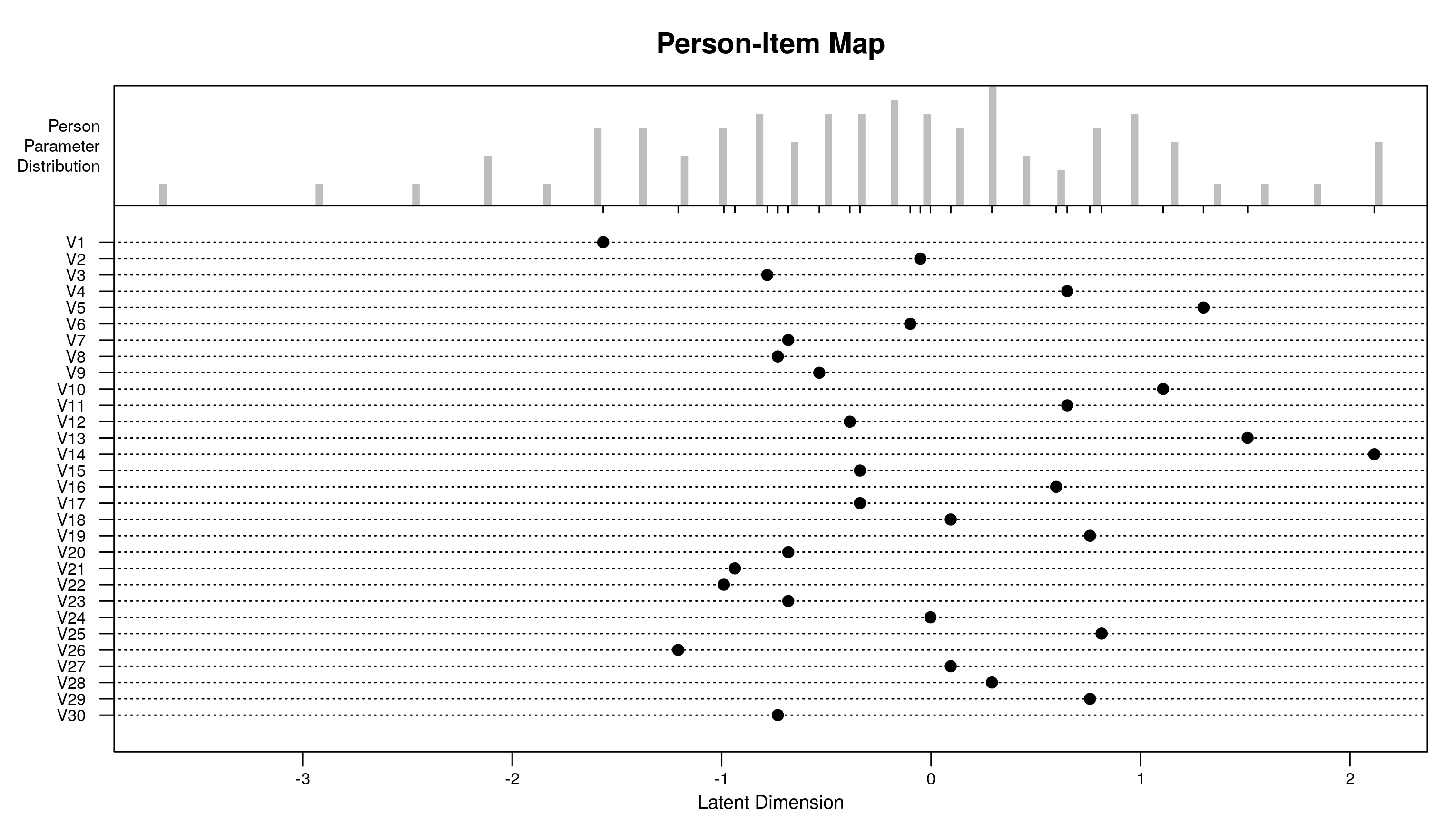
To create this map, we need item difficulties (regression coefficients * -1) and person abilities (random intercepts).
item.diff <- -1 * coef(summary(res.mlm.l))[, 1] # Regression coefficients * -1
item.diff[1] <- -1 * sum(item.diff[2:30]) # Difficulty of first item is sum of all others
item.diff <- data.frame(
  item.diff = as.numeric(item.diff), item = paste0("V", 1:30))
head(item.diff, 3) # What have we done?

    item.diff item
1 -1.56449994   V1
2 -0.05166222   V2
3 -0.78247594   V3

item.diff$move <- 1:30 # Cosmetic move to help me when creating PI chart

# For person abilities
pers.ab.df <- data.frame(pers.ability = ranef(res.mlm.l)$ID[, 1])

# GGPLOT-ING
ggplot(pers.ab.df, aes(x = pers.ability)) +
  geom_histogram(aes(y = ..count..), binwidth = .02, colour = 1) +
  geom_segment(mapping = aes(x = item.diff, xend = item.diff, yend = -.25),
               data = data.frame(item.diff), y = 0, linetype = 1) +
  geom_point(mapping = aes(x = item.diff, y = -.75 - move / 2),
            data = data.frame(item.diff), size = 1) +
  scale_y_continuous(breaks = c((-.75 + (-30:-1)/2), 0:8),
                     labels = c(paste0("V", 30:1), 0:8)) +
  geom_hline(yintercept = c(-.75 + seq(-29, 0, 2)/2), linetype = 3, size = .5) +
  geom_hline(yintercept = 0) +
  scale_x_continuous(breaks = seq(-4, 4, .5)) +
  labs(x = "Latent dimension", y = "", title = "Person-item map") +
  theme_classic() +
  geom_label(label = "Distribution of person ability", x = -1.8, y = 8) +
  theme(axis.title.y = element_text(hjust = 1))
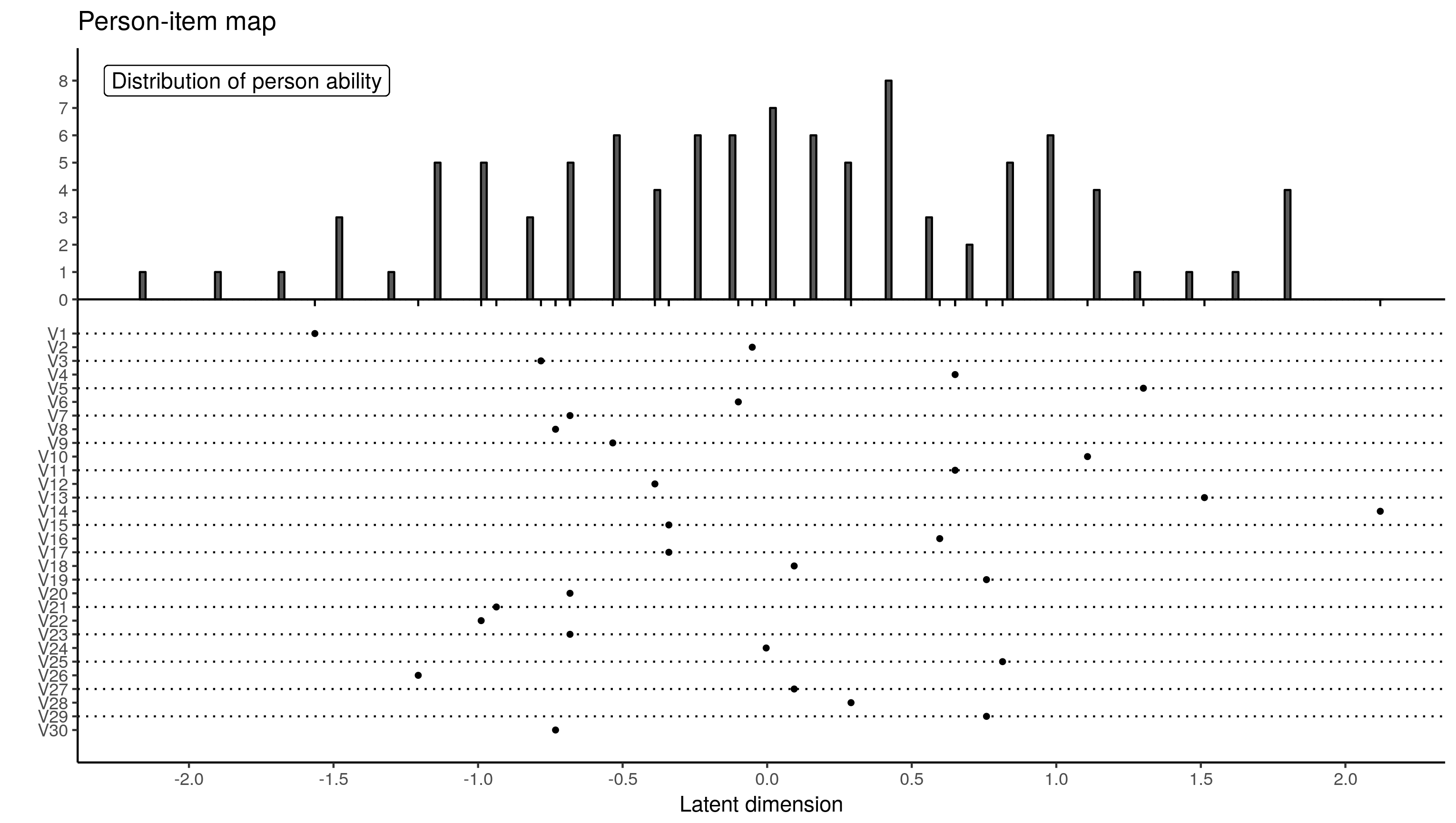
The extreme person scores are different. This is down to differences in MML and whatever method eRm uses to obtain person measures. It has to use a two-step process of sorts because CML does not provide person measures.
Item-Characteristic Curves
eRm provides a item characteristic curves with a single line:
plotjointICC(res.rasch)
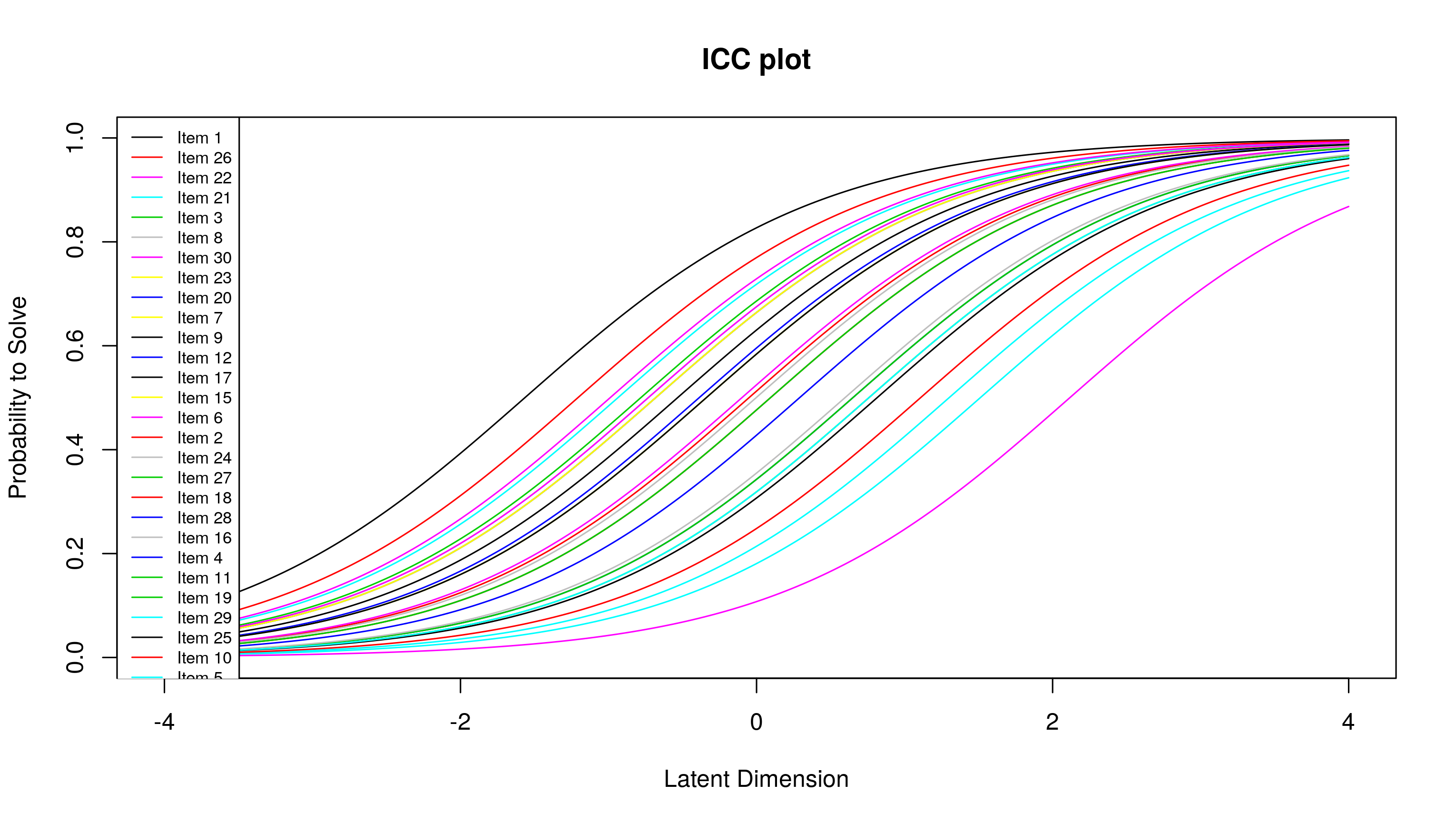
Here, we need to be able to predict the probability that a student will get an item correct, given their latent ability. What I did was use the logistic equation to predict probabilities. The log-odds given a latent ability is the difference between a latent ability and an item difficulty. Once this log-odds is obtained, calculating the predicted probability is easy. Since I’m using loops to do this, I also calculate item information, which is predicted probability multiplied by 1 - predicted probability. Here’s how:
{
  theta.s <- seq(-6, 6, .01) # Person abilities for prediction
  pred.prob <- c() # Vector to hold predicted probabilities
  test.info.df <- c() # Vector to hold test info
  for (i in theta.s) { # Loop through abilities
    for (j in 1:30) { # Loop through items
      l <- i - item.diff$item.diff[j] # log-odds is ability - difficulty
      l <- exp(-l) # Exponentiate -log-odds
      l <- 1 / (1 + l) # Calculate predicted probability
      pred.prob <- c(pred.prob, l) # Store predicted probability
      l <- l * (1 - l) # Calculate test information
      test.info.df <- c(test.info.df, l) # Store test information
    }
  }
  # Save it all to data frame
  test.info.df <- data.frame(
    theta = sort(rep(theta.s, 30)),
    item = rep(paste0("V", 1:30), length(theta.s)),
    info = test.info.df,
    prob = pred.prob,
    diff = item.diff$item.diff
  )
  rm(i, j, theta.s, pred.prob, l) # Clean environment
}

## GGPLOT-ING
ggplot(test.info.df, aes(x = theta, y = prob, colour = reorder(item, diff, mean))) +
  geom_line() +
  scale_y_continuous(labels = percent) +
  scale_x_continuous(breaks = -6:6, limits = c(-4, 4)) +
  labs(x = "Person ability", y = "Probability of correct response", colour = "Item",
       title = "Joint item characteristic plot") +
  theme_classic()
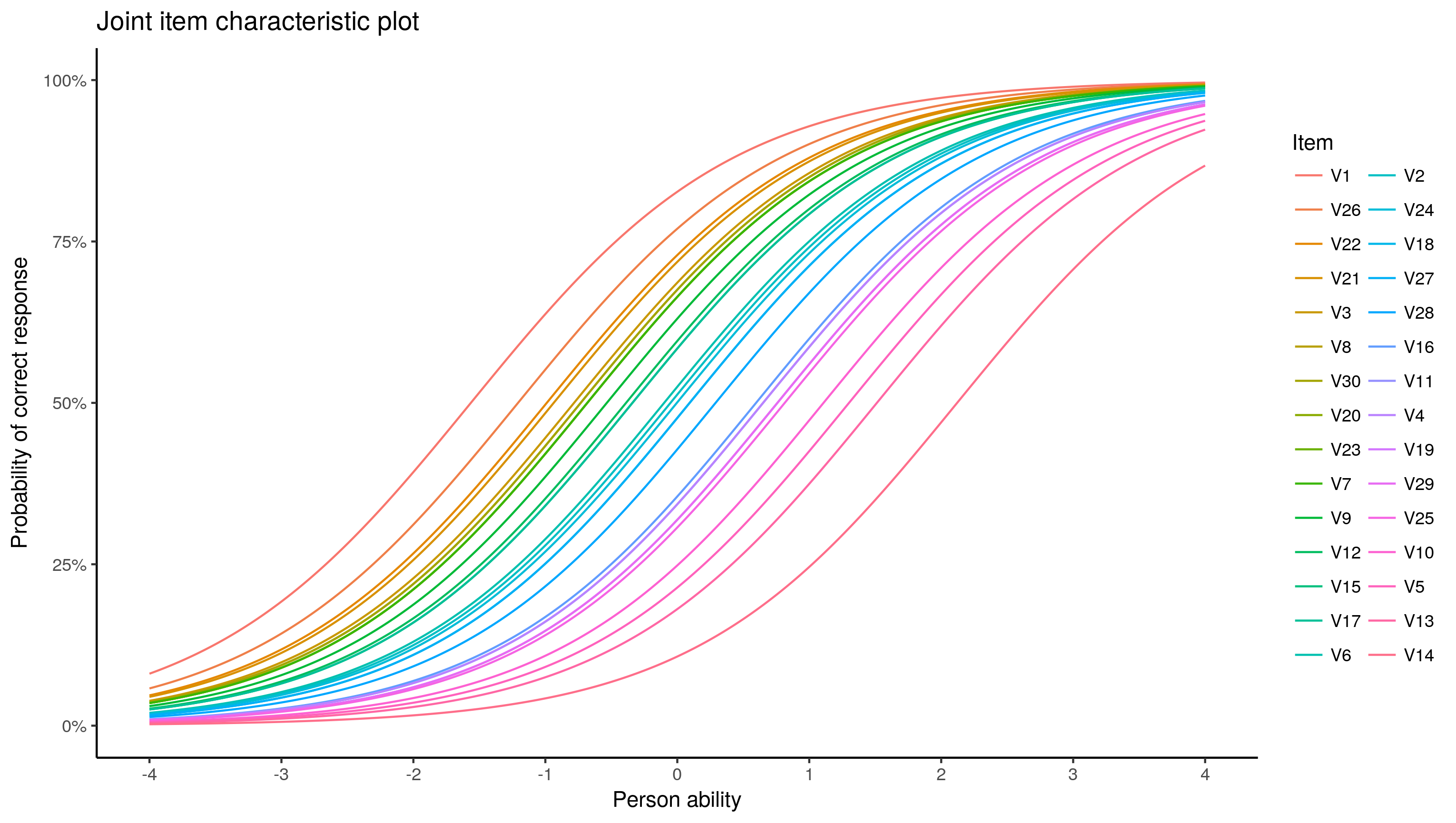
I find the colours ambiguous, the code below would produce an item by item plot, not printed
ggplot(test.info.df, aes(x = theta, y = prob)) + geom_line() +
  scale_x_continuous(breaks = seq(-6, 6, 2), limits = c(-4, 4)) +
  scale_y_continuous(labels = percent, breaks = seq(0, 1, .25)) +
  labs(x = "Person ability", y = "Probability of correct response",
       title = "Item characteristic plot",
       subtitle = "Items ordered from least to most difficult") +
  facet_wrap(~ reorder(item, diff, mean), ncol = 10) +
  theme_classic()
Person parameter plot
Again, a one-liner in eRm:
plot(person.parameter(res.rasch))
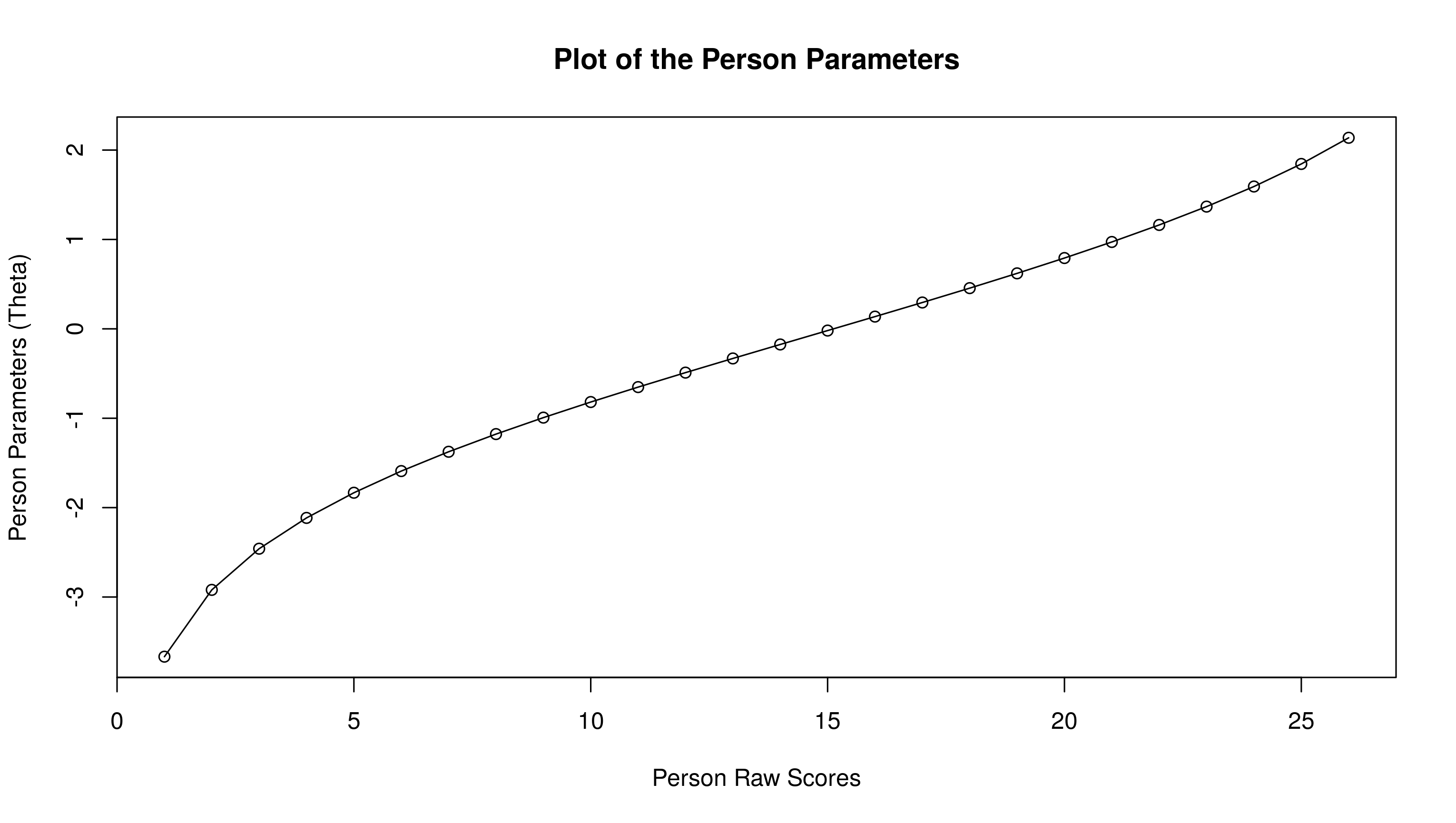
Compared to others, this is fairly straightforward. We need the estimated person abilities:
raschdat1.long$ability <- ranef(res.mlm.l)$ID[, 1]

# And GGPLOT-ING IT:
ggplot(raschdat1.long, aes(x = tot, y = ability)) +
  geom_point(shape = 1, size = 2) + geom_line() +
  scale_x_continuous(breaks = 1:26) +
  scale_y_continuous(breaks = round(c(
    min(raschdat1.long$ability),seq(-1.5, 1.5, .5),
    max(raschdat1.long$ability)), 2)) +
  labs(x = "Raw scores", y = "Latent scores", title = "Person parameter plot") +
  theme_classic()
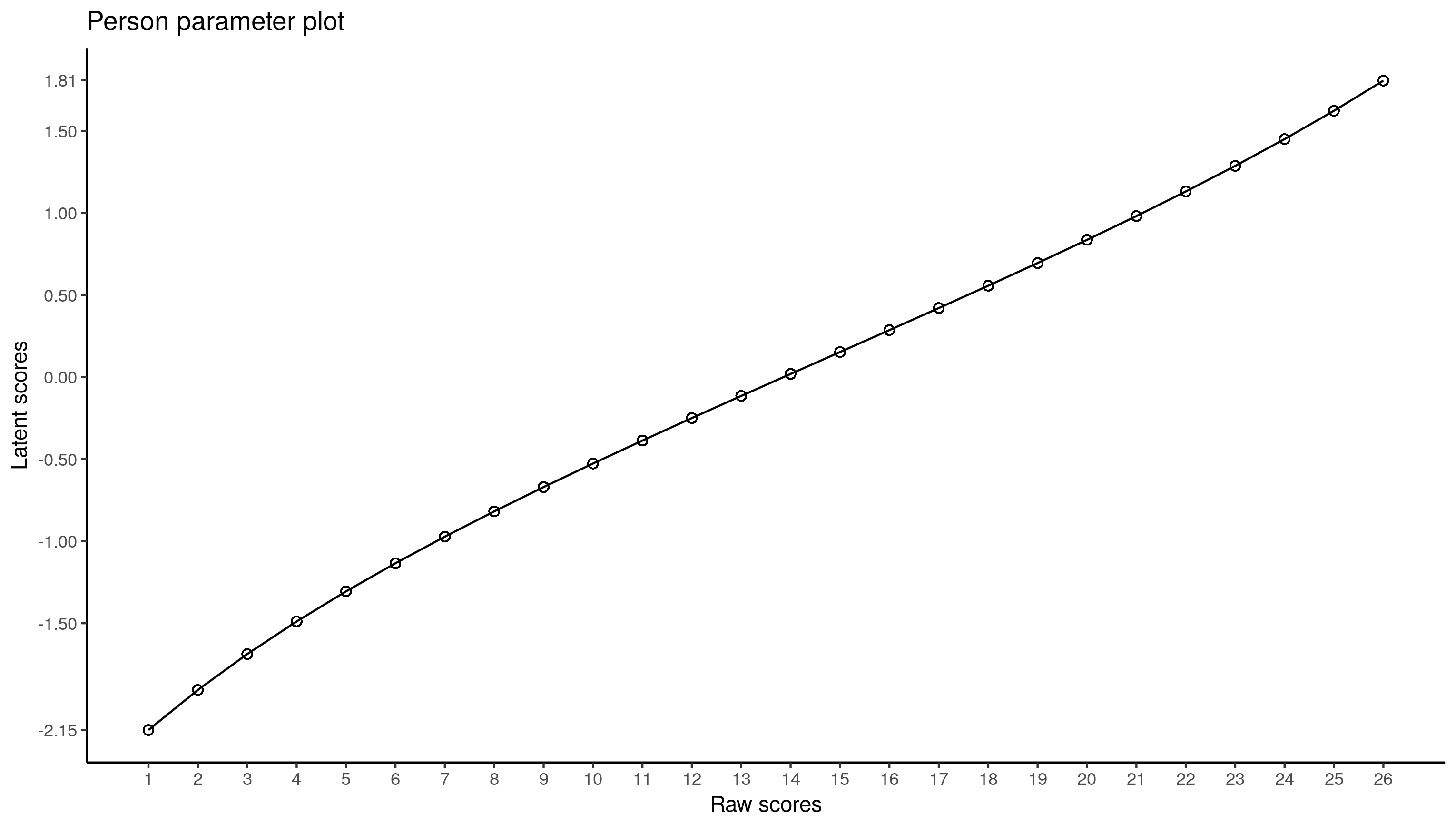
Both plots are not the same, though they overlap for the most part. Because estimation of person parameters is more tedious in CML, I’d trust the multilevel values.
Item fit using mean square
For the outfit MSQ, you square the residual (on the response scale, or actual score - predicted probability), and divide it by the predicted probability \(\times\) (1 - predicted probability). The average of this value for each item is its outfit mean square. The average of this value for each person is their outfit mean square.
For the infit MSQ, you perform the same computations. However, you perform these computations within the items for item infit, and within the persons for person infit. This is a vague; for some reason, I had issues typing out the formula in MathJax. See slides 14 and 15 here for formulae.
eRm one-liner:
itemfit(person.parameter(res.rasch)) # Not printed

# First, we need fitted and residual values
raschdat1.long$fitted <- fitted(res.mlm.l)
raschdat1.long$resid <- resid(res.mlm.l, type = "response")

# To calculate outfit MSQ:
raschdat1.long$o.msq <- (raschdat1.long$resid ^ 2) /
  (raschdat1.long$fitted * (1 - raschdat1.long$fitted))

# Summarize it by item using mean
item.diff$o.msq <- summarize(group_by(raschdat1.long, item),
                             o.msq = mean(o.msq))$o.msq

# To calculate infit MSQ:
item.diff$i.msq <- summarize(group_by(raschdat1.long, item), i.msq = sum(resid ^ 2) /
                              sum(fitted * (1 - fitted)))$i.msq

# Move everything into one data frame to compare using GGPLOT
{
  item.fit.df <- data.frame(
    item = paste0("V", 1:30), mml.osq = item.diff$o.msq, mml.isq = item.diff$i.msq,
    cml.osq = itemfit(person.parameter(res.rasch))$i.outfitMSQ,
    cml.isq = itemfit(person.parameter(res.rasch))$i.infitMSQ
  )
  item.fit.df <- cbind(
    tidyr::gather(item.fit.df[, 1:3], method.mml, mml, mml.osq:mml.isq),
    tidyr::gather(item.fit.df[, 4:5], method.cml, cml, cml.osq:cml.isq)
  )
  item.fit.df <- cbind(item.fit.df[, c(1, 3, 5)], method = c(
    rep("Outfit MSQ", 30), rep("Infit MSQ", 30)))
}

ggplot(item.fit.df, aes(x = mml, y = cml)) +
  scale_x_continuous(breaks = seq(0, 2, .1)) +
  scale_y_continuous(breaks = seq(0, 2, .1)) +
  geom_point(shape = 1) + geom_abline(slope = 1) + theme_classic() +
  geom_smooth(se = FALSE) + facet_wrap(~ method, ncol = 2) +
  labs(x = "glmer (MML)", y = "eRm (CML)", title = "Item fit comparing CML and MML")
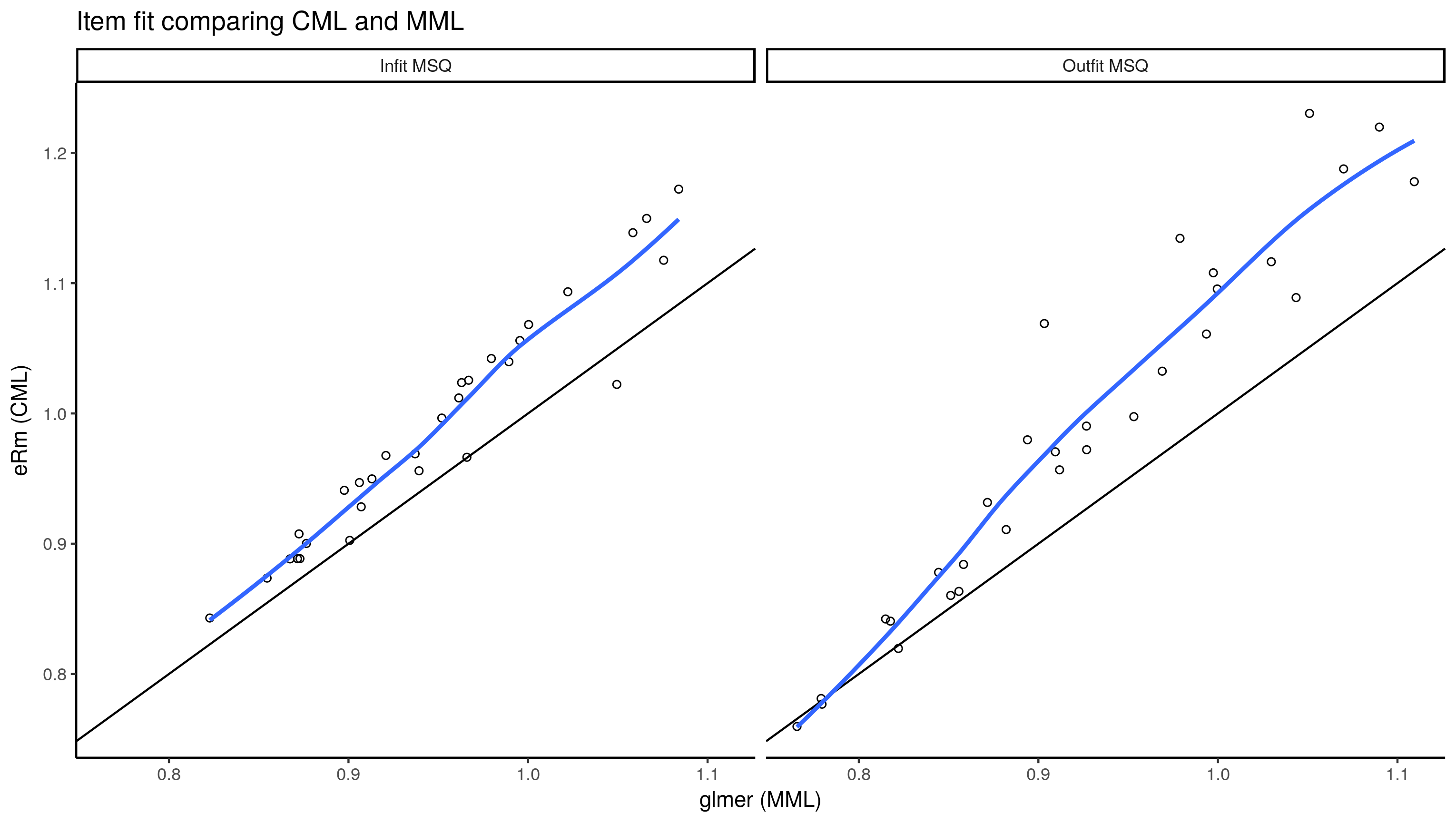
Interestingly, it seems the MSQ from CML is almost always higher than that from the multilevel model (MML).
Person fit using mean square
eRm one-liner:
personfit(person.parameter(res.rasch)) # Not printed

pers.ab.df$ID <- 1:100

# Person outfit MSQ:
pers.ab.df$o.msq <- summarize(group_by(raschdat1.long, ID), o.msq = mean(o.msq))$o.msq

# Person infit MSQ:
pers.ab.df$i.msq <- summarize(group_by(raschdat1.long, ID), i.msq = sum(resid ^ 2) /
                                sum(fitted * (1 - fitted)))$i.msq

# Move everything into one data frame to compare using GGPLOT
{
  person.fit.df <- data.frame(
    ID = 1:100, mml.osq = pers.ab.df$o.msq, mml.isq = pers.ab.df$i.msq,
    cml.osq = personfit(person.parameter(res.rasch))$p.outfitMSQ,
    cml.isq = personfit(person.parameter(res.rasch))$p.infitMSQ
  )
  person.fit.df <- cbind(
    tidyr::gather(person.fit.df[, 1:3], method.mml, mml, mml.osq:mml.isq),
    tidyr::gather(person.fit.df[, 4:5], method.cml, cml, cml.osq:cml.isq)
  )
  person.fit.df <- cbind(person.fit.df[, c(1, 3, 5)], method = c(
    rep("Outfit MSQ", 100), rep("Infit MSQ", 100)))
}

ggplot(person.fit.df, aes(x = mml, y = cml)) +
  scale_x_continuous(breaks = seq(0, 2, .1)) +
  scale_y_continuous(breaks = seq(0, 2, .1)) +
  geom_point(shape = 1) + geom_abline(slope = 1) + theme_classic() +
  geom_smooth(se = FALSE) + facet_wrap(~ method, ncol = 2) +
  geom_text_repel(aes(
    label = ifelse(cml >= 1.5 | mml >= 1.5 | cml <= 0.5 | mml <= 0.5, ID, ""))) +
  geom_hline(yintercept = c(.5, 1.5), linetype = 2) +
  geom_vline(xintercept = c(.5, 1.5), linetype = 2) +
  labs(x = "glmer (MML)", y = "eRm (CML)", title = "Person fit comparing CML and MML")
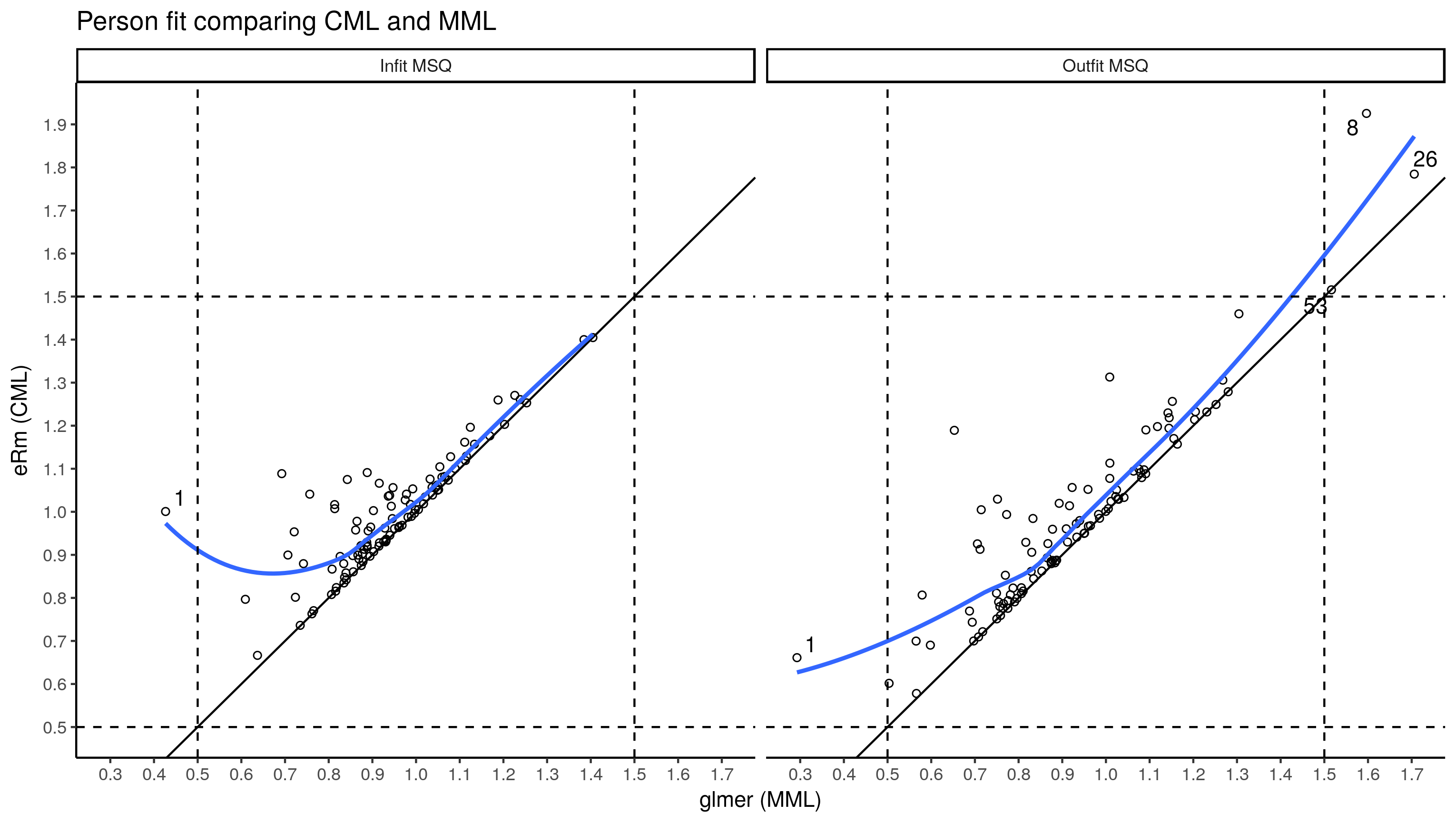
Same pattern, MSQ from CML is almost always higher than that from the multilevel model (MML) I used the conventional cut-offs to identify misfitting persons. Person 1 with low infit and outfit MSQ got only one question correct, cannot recall what stood out about 8, 26 and 53.
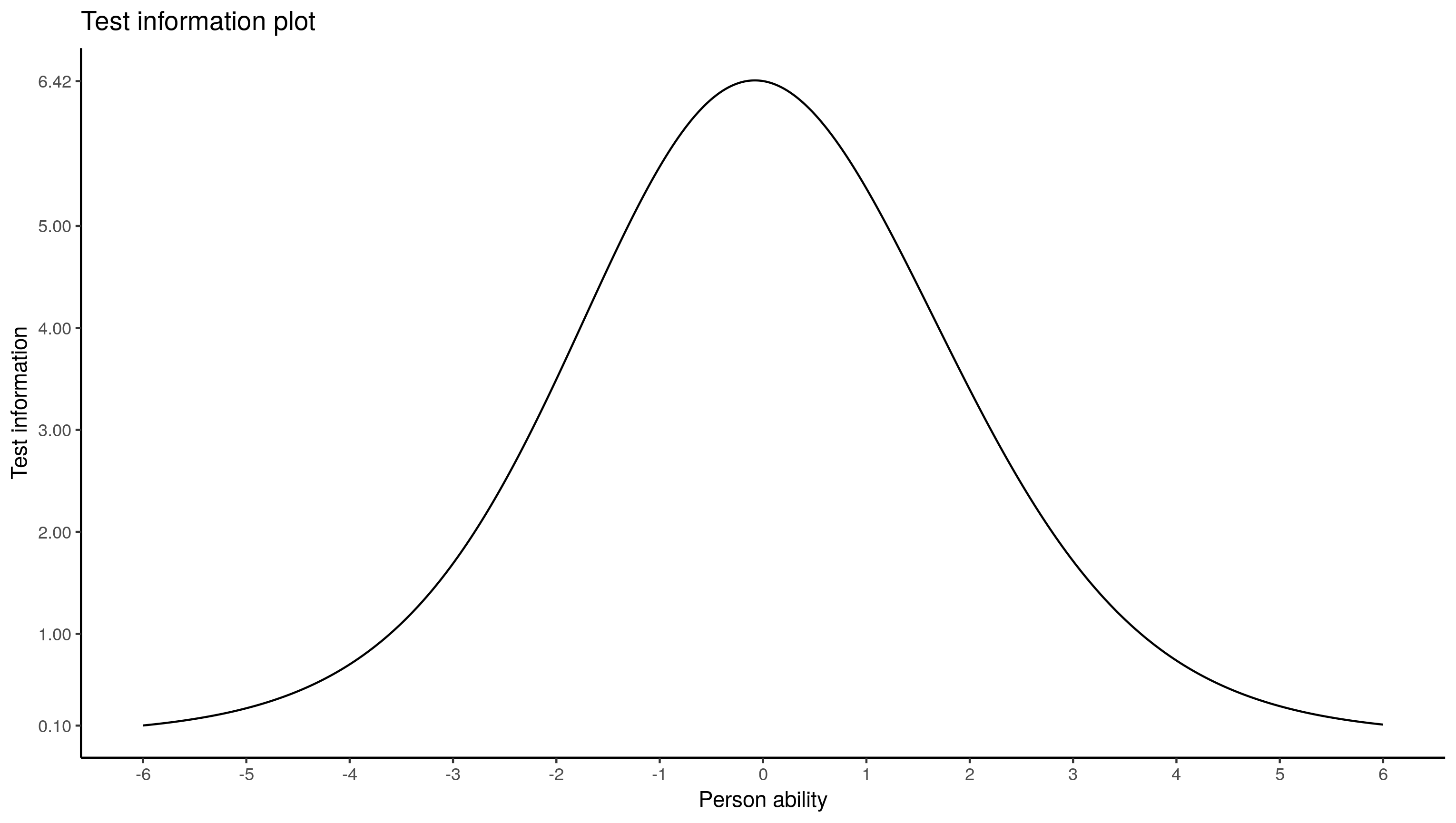
Test information
eRm one-liner:
plotINFO(res.rasch)
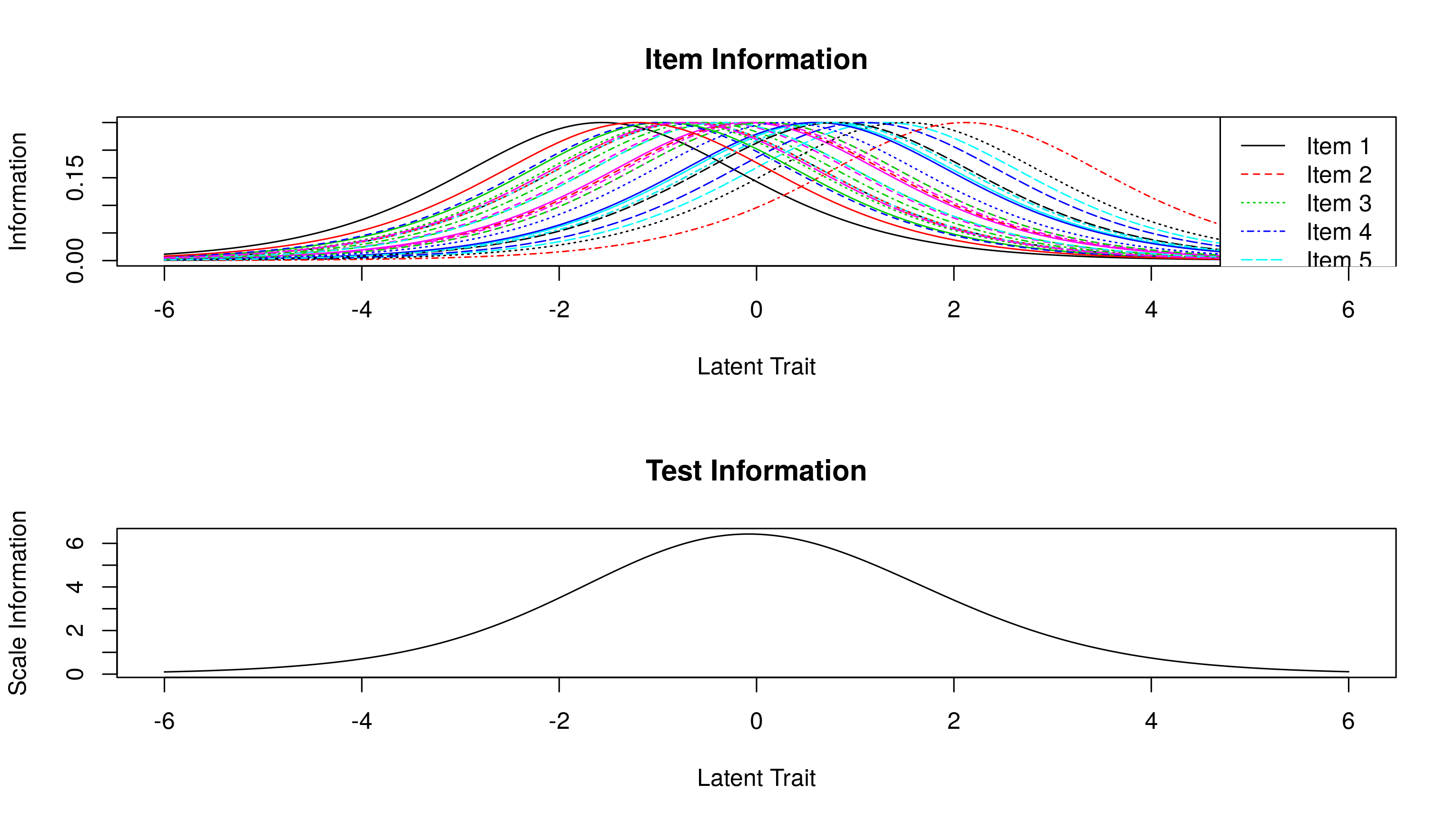
We’ve already done the work for this above when we created the ICCs, and calculated the test information. All that remains is plotting. For the overall test information, we need to sum each item’s test information:
ggplot(summarise(group_by(test.info.df, theta), info = sum(info)),
       aes(x = theta, y = info)) + geom_line() +
  scale_x_continuous(breaks = -6:6) +
  scale_y_continuous(breaks = c(1:5, .10, 6.42)) +
  labs(x = "Person ability", y = "Test information", colour = "Item",
       title = "Test information plot") +
  theme_classic()
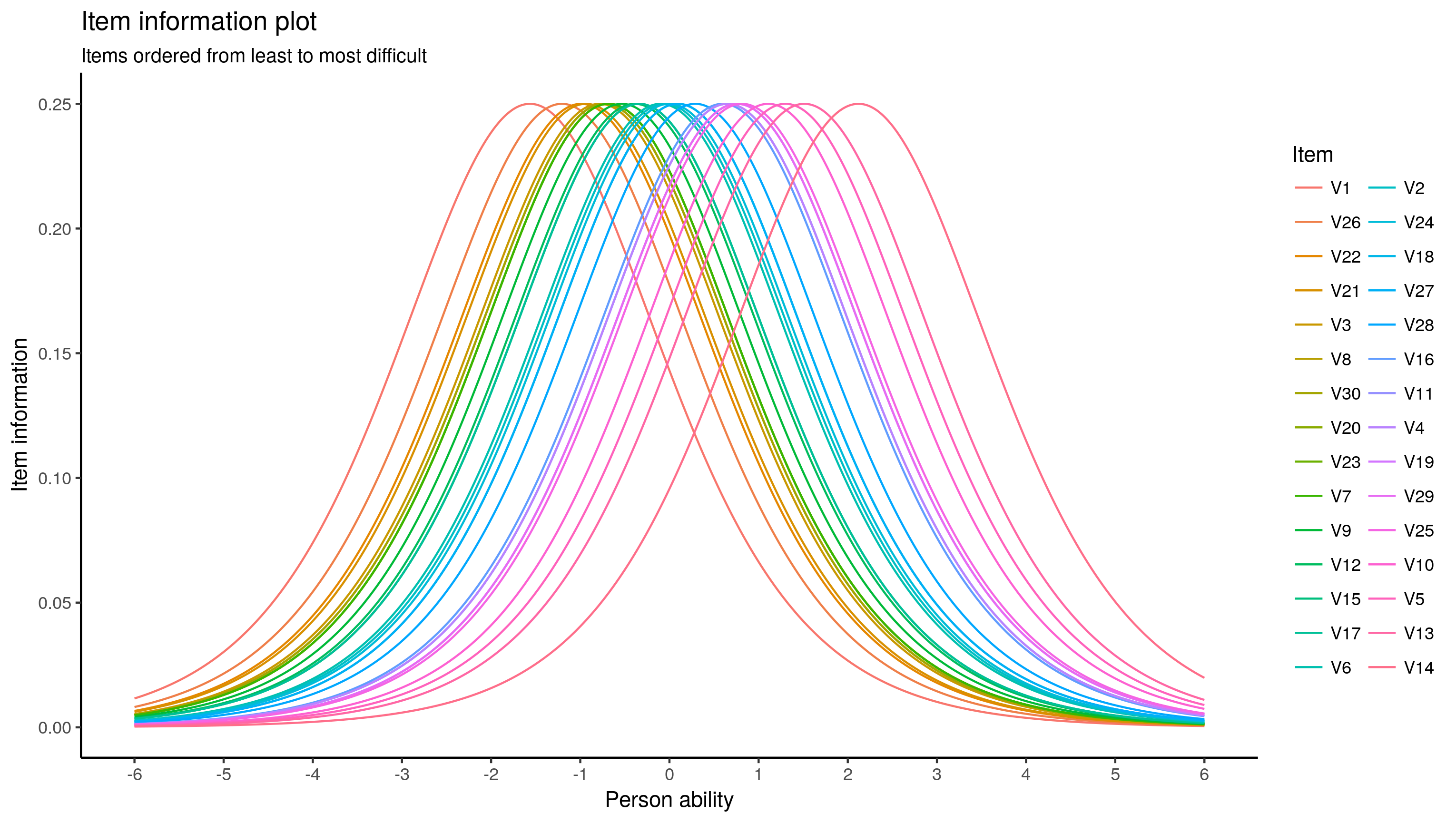
# And the ambiguous colour plot:
ggplot(test.info.df, aes(x = theta, y = info)) +
  geom_line(aes(colour = reorder(item, diff, mean))) +
  scale_x_continuous(breaks = seq(-6, 6, 1)) +
  labs(x = "Person ability", y = "Item information", colour = "Item",
       title = "Item information plot",
       subtitle = "Items ordered from least to most difficult") +
  theme_classic()
And finally, using the Standard Error of Measurement (SEM), I thought you could create a confidence-band like plot. The SEM is the inverse of the root of test information.
ggplot(summarise(group_by(test.info.df, theta), info = 1 / sqrt(sum(info))),
       aes(x = theta)) +
  scale_x_continuous(breaks = seq(-3, 3, 1), limits = c(-3, 3)) +
  scale_y_continuous(breaks = c(seq(-3, 3, 1), -4.5, 4.5), limits = c(-4.5, 4.5)) +
  geom_line(aes(y = theta), size = .5) +
  geom_errorbar(aes(ymin = -1.96 * info + theta, ymax = 1.96 * info + theta), size = .05) +
  labs(x = "Estimated person ability", y = "Range of 95% of true scores") +
  geom_hline(yintercept = c(seq(-3, 3, 1), -4.5, 4.5), linetype = 1, size = .05) +
  theme_classic()
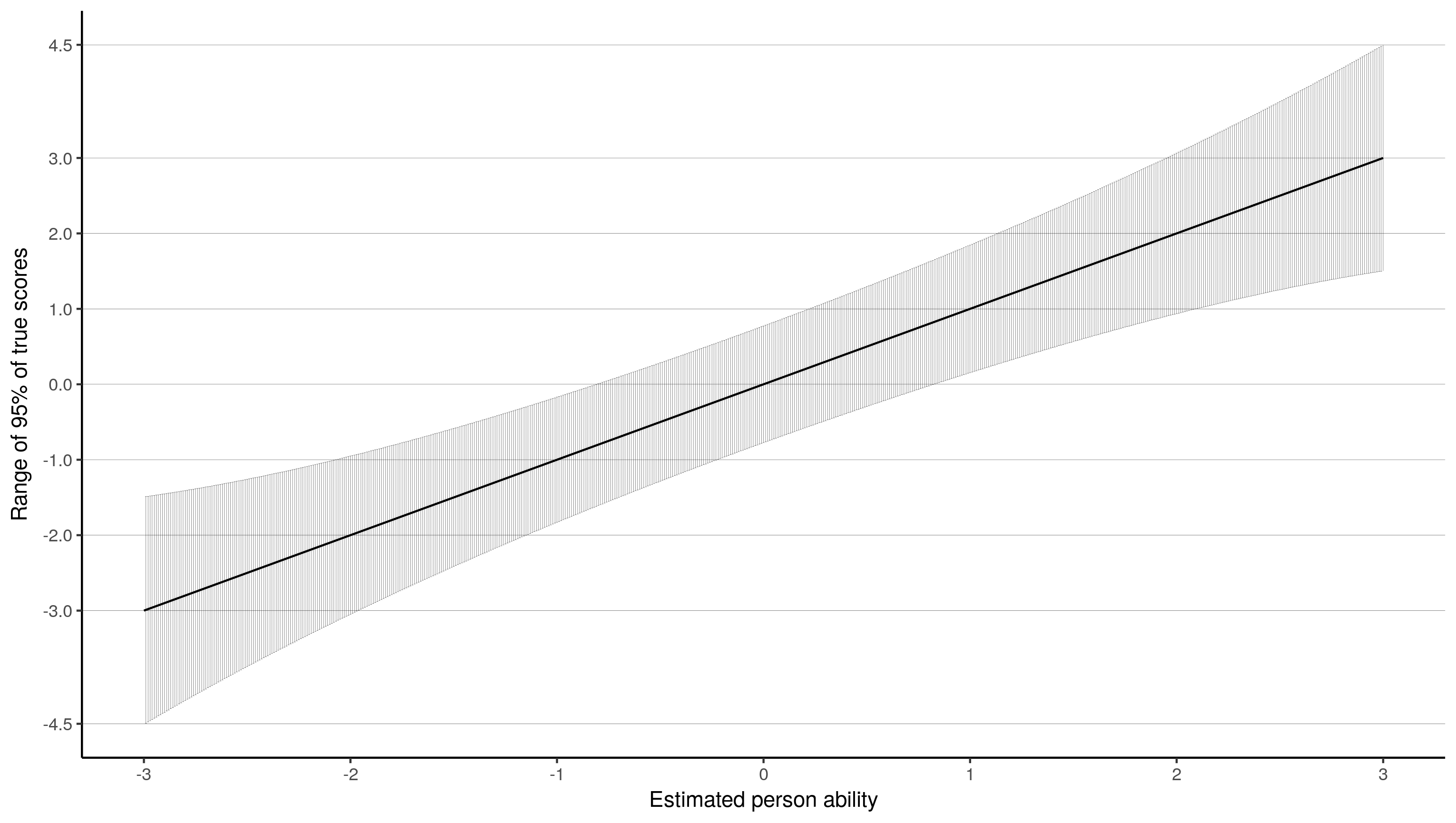
This is the one I like best, because I feel it is most informative. This plot shows that for a kid with an estimated ability of -3, their ability is estimated with such precision that their actual score could lie between -1.5 and -4.5. In the middle at 0, the actual score could lie between, by my guess, -.8 and .8. I am not so sure this interpretation is correct, but it is appealing :).
I’m not sure what I have achieved here, apart from a lot of ggplot-ing, … But having worked through this, I feel I can better understand what the model is trying to claim a series of items, and what some of its diagnostics are about. Also, because the model is a regression model, it is set for the addition of additional predictors - but that’s no longer a Rasch model. I guess the next step would be to replicate this on real data I am working on. The vcrpart & ordinal packages could work for this, as it performs ordinal multilevel regression. However, ordinal only performs cumulative link logistic regression (Rijmen et al.1 call it the graded response model), while vcrpart performs cumulative link, adjacent categories (partial credit model and rating scale model), and baseline category (nominal response model) ordinal regression models.
I have left out differential item functioning, but I believe that to be testing the fixed effects of groups in the data, and testing the interaction between test items and groups.2
P.S.: Rasch analysis is not just math (multilevel logistic regression, conditional logistic regression), it also seems to be a philosophy. So I guess the title here is misleading :). I have not used glmer() to perform Rasch analysis, I just created the outputs that support Rasch analysis.
-
Rijmen, F., Tuerlinckx, F., De Boeck, P., & Kuppens, P. (2003). A nonlinear mixed model framework for item response theory. Psychological Methods, 8(2), 185–205. https://doi.org/10.1037/1082-989X.8.2.185 ↩︎
-
De Boeck, P., Bakker, M., Zwitser, R., Nivard, M., Hofman, A., Tuerlinckx, F., & Partchev, I. (2011). The Estimation of Item Response Models with the lmer Function from the lme4 Package in R. Journal Of Statistical Software, 39(12), 1–28. https://doi.org/10.18637/jss.v039.i12 ↩︎
-
Hedeker, D., Mermelstein, R. J., Demirtas, H., & Berbaum, M. L. (2016). A mixed-effects location-scale model for ordinal questionnaire data. Health Services and Outcomes Research Methodology, 16(3), 117–131. https://doi.org/10.1007/s10742-016-0145-9 ↩︎
-
Engec, N. (1998). Logistic regression and item response theory: Estimation item and ability parameters by using logistic regression in IRT. ProQuest Dissertations and Theses. Retrieved from http://digitalcommons.lsu.edu/gradschool_disstheses/6731 ↩︎
-
Reise, S. P. (2000). Using mutlilevel logistic regression to evaluate person-fit in IRT models. Multivariate Behavioral Research, 35(4), 543–568. https://doi.org/10.1207/S15327906MBR3504_06 ↩︎
-
De Boeck, P., & Wilson, M. (2004). Explanatory item response models : a generalized linear and nonlinear approach. (P. De Boeck & M. Wilson, Eds.). New York, NY: Springer New York. https://doi.org/10.1007/978-1-4757-3990-9 ↩︎
Comments powered by Talkyard.