TLDR: If you have good measurement quality, conventional benchmarks for fit indices may lead to bad decisions. Additionally, global fit indices are not informative for investigating misspecification.
I am working with one of my professors, Dr. Jessica Logan, on a checklist for the developmental progress of young children. We intend to take this down the IRT route (or ordinal logistic regression), but currently, this is all part of a factor analysis course project. So I ran some CFA models, and was discussing model fit with Dr. Logan. I commented that factor loadings were generally high (1st quartile = .80, M/Mdn = .84), but initial model fit was inadequate to play the model fit game, for example, RMSEA > .06, … She commented that she was not so worried by this combination: high loadings together with failure to meet conventional model fit guidelines. And pointed me towards a recent paper by Dan McNeish, Ji An and Gregory Hancock,1 hereafter MAH, - the paper is available on ResearchGate.
MAH’s argument hinges on an important point: all models are usually misspecified in practice. Counterintuitively, holding misspecification constant, models with lower factor loadings (or poorer measurement quality) have better fit indices than models with higher factor loadings. For example, if two models have the same level of misspecification, and one with factor loadings of .9 could have RMSEA higher than .2, and a model with factor loadings of .4 could have RMSEA less than .05. The paper contains some charts that communicate these results very clearly.
And this is why in their conclusion, MAH write:
By comparison, if one is researching a construct for which very high measurement quality can be obtained, one need not subscribe to such stringent AFI criteria to be confident that the model features any nontrivial misspecifications. Conversely, if one is researching a construct that cannot be measured very reliably, the currently employed cutoffs are not suitable and would be very likely to overlook potentially meaningful misspecifications in the model.
AFIs are approximate goodness of fit indices, these include absolute fit indices like the RMSEA and SRMR, and relative fit indices like CFI.
An alternative to working with global fit indices
The fit indices MAH write about are global fit indices (hereafter GFIs) and they detect all types of model misspecifications. However, as MAH point out, not all model misspecifications are problematic. Consider order effects, two items may have correlated errors independent of their shared factor simply because one follows the other (serial correlation). The absence of this correlated error in a CFA (the default) would negatively impact any global fit index. Moreover, global fit indices do not tell you what your model misspecifications are.
The sections that follow may include details that not everyone would like to read about, you can skip to the bottom of the page for annotated lavaan code for what to do instead of using global fit indices.
MAH reference a 2009 paper by Satis, Satorra and van der Veld,2 hereafter SSV, that addresses this issue. SSV laid out a method for investigating model misspecifications that involves the use of modification indices (MI), expected parameter change (EPC), theory and power analysis. The EPC is the value by which a constrained relationship would change from zero if it was freed to be estimated by the model. I believe researchers are familiar with MIs and often use them to fix model misspecifications with the aim of obtaining GFIs that their reviewers will accept. The relationship between MI and EPC is:
$$MI = (EPC/\sigma)^2$$
where \(\sigma\) is the standard error of the EPC.
SSV suggest the following framework:
- specify an unacceptable level of model misspecification \((\delta)\) for any constrained relationship in your model. They recommend thinking about your context, or:
- for factor loadings, absolute value > .4
- for correlated errors, absolute value > .1
- calculate a noncentrality parameter, \(ncp=(\delta/\sigma)^2\)
- this \(ncp\) follows a noncental-\(\chi^2\) distribution which you can use to calculate the statistical power to detect \(\delta\), the unnaceptable degree of model misspecification, for each constrained relationship.
Next, the following decision rules:
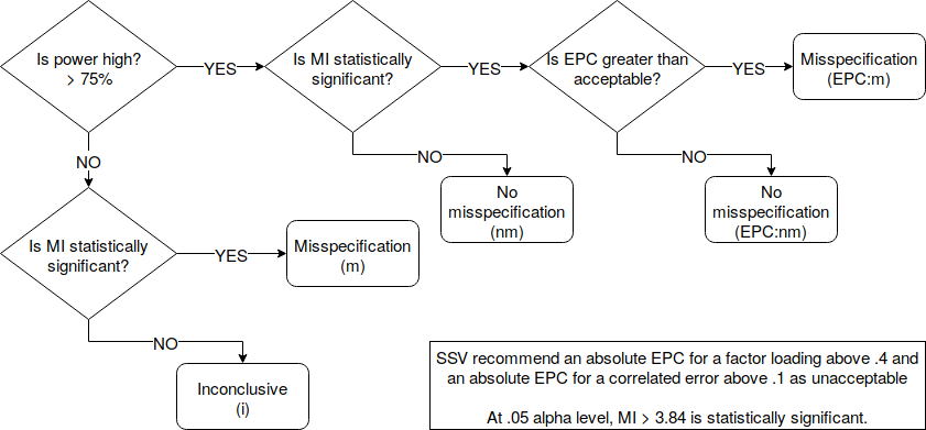
The nice thing is this is all implemented in lavaan in R. Misspecification codes:
- Model misspecification:
(m),(EPC:m) - No model misspecification:
(nm),(EPC:nm) - Inconclusive on model misspecification:
(i)
library(lavaan)
For this, I’ll assume HolzingerSwineford1939 data are 9 questions, and the respondents answered them x1 to x9 sequentially.
data("HolzingerSwineford1939")
# model syntax for HolzingerSwineford1939 dataset
(syntax <- paste(
  paste("f1 =~", paste0("x", 1:3, collapse = " + ")),
  paste("f2 =~", paste0("x", 4:6, collapse = " + ")),
  paste("f3 =~", paste0("x", 7:9, collapse = " + ")),
  sep = "\n"))

[1] "f1 =~ x1 + x2 + x3\nf2 =~ x4 + x5 + x6\nf3 =~ x7 + x8 + x9"
Run model, standardize latent variables, & report standardized results:
summary(hs.fit <- cfa(syntax, HolzingerSwineford1939, std.lv = TRUE),
        standardize = TRUE)

lavaan (0.5-23.1097) converged normally after  22 iterations

  Number of observations                           301

  Estimator                                         ML
  Minimum Function Test Statistic               85.306
  Degrees of freedom                                24
  P-value (Chi-square)                           0.000

Parameter Estimates:

  Information                                 Expected
  Standard Errors                             Standard

Latent Variables:
                   Estimate  Std.Err  z-value  P(>|z|)   Std.lv  Std.all
  f1 =~
    x1                0.900    0.081   11.127    0.000    0.900    0.772
    x2                0.498    0.077    6.429    0.000    0.498    0.424
    x3                0.656    0.074    8.817    0.000    0.656    0.581
  f2 =~
    x4                0.990    0.057   17.474    0.000    0.990    0.852
    x5                1.102    0.063   17.576    0.000    1.102    0.855
    x6                0.917    0.054   17.082    0.000    0.917    0.838
  f3 =~
    x7                0.619    0.070    8.903    0.000    0.619    0.570
    x8                0.731    0.066   11.090    0.000    0.731    0.723
    x9                0.670    0.065   10.305    0.000    0.670    0.665

Covariances:
                   Estimate  Std.Err  z-value  P(>|z|)   Std.lv  Std.all
  f1 ~~
    f2                0.459    0.064    7.189    0.000    0.459    0.459
    f3                0.471    0.073    6.461    0.000    0.471    0.471
  f2 ~~
    f3                0.283    0.069    4.117    0.000    0.283    0.283

Variances:
                   Estimate  Std.Err  z-value  P(>|z|)   Std.lv  Std.all
   .x1                0.549    0.114    4.833    0.000    0.549    0.404
   .x2                1.134    0.102   11.146    0.000    1.134    0.821
   .x3                0.844    0.091    9.317    0.000    0.844    0.662
   .x4                0.371    0.048    7.778    0.000    0.371    0.275
   .x5                0.446    0.058    7.642    0.000    0.446    0.269
   .x6                0.356    0.043    8.277    0.000    0.356    0.298
   .x7                0.799    0.081    9.823    0.000    0.799    0.676
   .x8                0.488    0.074    6.573    0.000    0.488    0.477
   .x9                0.566    0.071    8.003    0.000    0.566    0.558
    f1                1.000                               1.000    1.000
    f2                1.000                               1.000    1.000
    f3                1.000                               1.000    1.000
Chi-square is statistically significant, there is at least some misfit
Request modification indices. Sort them from highest to lowest. Do not print any MI below 3 for convenience of presentation. Apply SSV method by requesting power = TRUE, and setting delta. delta for those who skipped is unacceptable level of misfit, so a delta = .4 standard for factor loadings means I care about the factor loading if it is missing from my model and its factor loading is greater than .4. By default, delta = .1 in lavaan. Based on SSV’s recommendations, this is adequate for correlated errors. So I select only correlated errors for output using op = "~~".
modificationindices(hs.fit, sort. = TRUE, minimum.value = 3, power = TRUE,
                    op = "~~")


lhs op rhs        mi    epc sepc.all delta   ncp power decision
30  f1 =~  x9 36.411  0.519    0.515   0.1 1.351 0.213  **(m)**
76  x7 ~~  x8 34.145  0.536    0.488   0.1 1.187 0.193  **(m)**
28  f1 =~  x7 18.631 -0.380   -0.349   0.1 1.294 0.206  **(m)**
78  x8 ~~  x9 14.946 -0.423   -0.415   0.1 0.835 0.150  **(m)**
33  f2 =~  x3  9.151 -0.269   -0.238   0.1 1.266 0.203  **(m)**
55  x2 ~~  x7  8.918 -0.183   -0.143   0.1 2.671 0.373  **(m)**
31  f2 =~  x1  8.903  0.347    0.297   0.1 0.741 0.138  **(m)**
51  x2 ~~  x3  8.532  0.218    0.164   0.1 1.791 0.268  **(m)**
59  x3 ~~  x5  7.858 -0.130   -0.089   0.1 4.643 0.577  **(m)**
26  f1 =~  x5  7.441 -0.189   -0.147   0.1 2.087 0.303  **(m)**
50  x1 ~~  x9  7.335  0.138    0.117   0.1 3.858 0.502  **(m)**
65  x4 ~~  x6  6.221 -0.235   -0.185   0.1 1.128 0.186  **(m)**
66  x4 ~~  x7  5.920  0.098    0.078   0.1 6.141 0.698  **(m)**
48  x1 ~~  x7  5.420 -0.129   -0.102   0.1 3.251 0.438  **(m)**
77  x7 ~~  x9  5.183 -0.187   -0.170   0.1 1.487 0.230  **(m)**
36  f2 =~  x9  4.796  0.137    0.136   0.1 2.557 0.359  **(m)**
29  f1 =~  x8  4.295 -0.189   -0.187   0.1 1.199 0.195  **(m)**
63  x3 ~~  x9  4.126  0.102    0.089   0.1 3.993 0.515  **(m)**
67  x4 ~~  x8  3.805 -0.069   -0.059   0.1 7.975 0.806     (nm)
43  x1 ~~  x2  3.606 -0.184   -0.134   0.1 1.068 0.178      (i)
45  x1 ~~  x4  3.554  0.078    0.058   0.1 5.797 0.673      (i)
35  f2 =~  x8  3.359 -0.120   -0.118   0.1 2.351 0.335      (i)
Check the decision column. x7 and x8 is termed misspecification because power is low at .193, yet the MI is statistically significant. However, this may simply be due to order effects, and such misspecification may be acceptable. I will not add this correlated error to my model. Same goes for x8 and x9 (lhs 78) and x2 and x3 (lhs 51). These missing serial-correlations are acceptable misspecifications.
However consider x2 and x7 (lhs 55), low power at .373 yet significant MI. Is there some theory connecting these two items? Can I explain the suggested correlation?
Consider x4 and x8 (lhs 67), high power at .806, yet the MI is not statistically significant, hence we can conclude there is no misspecification.
Consider x1 and x4 (lhs 45), low power at .673, and the MI is not statistically significant, hence this is inconclusive.
Now for the factor loadings:
modificationindices(hs.fit, sort. = TRUE, power = TRUE, delta = .4, op = "=~")

lhs op rhs        mi    epc sepc.all delta    ncp power decision
30  f1 =~  x9 36.411  0.519    0.515   0.4 21.620 0.996  *epc:m*
28  f1 =~  x7 18.631 -0.380   -0.349   0.4 20.696 0.995   epc:nm
33  f2 =~  x3  9.151 -0.269   -0.238   0.4 20.258 0.994   epc:nm
31  f2 =~  x1  8.903  0.347    0.297   0.4 11.849 0.931   epc:nm
26  f1 =~  x5  7.441 -0.189   -0.147   0.4 33.388 1.000   epc:nm
36  f2 =~  x9  4.796  0.137    0.136   0.4 40.904 1.000   epc:nm
29  f1 =~  x8  4.295 -0.189   -0.187   0.4 19.178 0.992   epc:nm
35  f2 =~  x8  3.359 -0.120   -0.118   0.4 37.614 1.000     (nm)
27  f1 =~  x6  2.843  0.100    0.092   0.4 45.280 1.000     (nm)
38  f3 =~  x2  1.580 -0.123   -0.105   0.4 16.747 0.984     (nm)
25  f1 =~  x4  1.211  0.069    0.059   0.4 40.867 1.000     (nm)
39  f3 =~  x3  0.716  0.084    0.075   0.4 16.148 0.980     (nm)
42  f3 =~  x6  0.273  0.027    0.025   0.4 58.464 1.000     (nm)
41  f3 =~  x5  0.201 -0.027   -0.021   0.4 43.345 1.000     (nm)
34  f2 =~  x7  0.098 -0.021   -0.019   0.4 36.318 1.000     (nm)
32  f2 =~  x2  0.017 -0.011   -0.010   0.4 21.870 0.997     (nm)
37  f3 =~  x1  0.014  0.015    0.013   0.4  9.700 0.876     (nm)
40  f3 =~  x4  0.003 -0.003   -0.003   0.4 52.995 1.000     (nm)
See the first line, suggesting I load x9 on f1. The power is high, the MI is significant and the EPC is higher than .4 suggesting that this is some type of misspecification that we should pay attention to.
However, the next line suggests I load x7 on f1. The power is high, the MI is significant, but the EPC is .38, less than .4, suggesting that we do not consider this misspecification to be high enough to warrant modifying the model. Same goes for a number of suggested modifications with decision epc:nm.
Then there is a final group with high power, but the MIs are not statistically significant, so we can conclude there is no misspecification.
Note that you can also tell lavaan what constitutes high power using the high.power = argument. 75% is what SSV use and is lavaan’s default but you can be flexible.
Note that you make only one change to the model at a time. The EPC and MI, are calculated assuming other parameters are approximately correct, hence the way to run the steps above is to make one change, then re-request the MIs, EPC, and power from lavaan.
I believe this is the approach recommended by SSV, and following this approach would cause one to think about the model when using MIs, while taking statistical power to detect misspecification into account. It is possible to resolve all the non-inconclusive relationships (using theory, modifications, …) and be left with a model where you do not have the power to detect the remaining misspecifications (a bunch of inconclusives). This would be another reason to reduce our confidence in our final modeling results.
P.S.: Another approach to latent variable modeling is PLS path modeling. It is a method for SEMs based on OLS regression. It stems from the work of Hermann Wold. Wold was Joreskog’s (LISREL) advisor, Joreskog was Muthen’s (Mplus) advisor. This is why my title uses covariance-based SEM instead of latent variable models or just SEMs.
-
McNeish, D., An, J., & Hancock, G. R. (2017). The Thorny Relation Between Measurement Quality and Fit Index Cutoffs in Latent Variable Models. Journal of Personality Assessment. https://doi.org/10.1080/00223891.2017.1281286 ↩︎
-
Saris, W. E., Satorra, A., & van der Veld, W. M. (2009). Testing Structural Equation Models or Detection of Misspecifications? Structural Equation Modeling: A Multidisciplinary Journal, 16(4), 561–582. https://doi.org/10.1080/10705510903203433 ↩︎
Comments powered by Talkyard.